Baseball ProGUESTus: Casting Some Uncertainty on How Players Age

Part One

You can’t predict baseball.

Have you ever thought about the distressing fact that nobody can predict the exact path along which a baseball will fly? I’m not trying to get in a fight with Profs. David Kagan, Alan Nathan, Meredith Wills, and folks like them. They have, among other talents, very large and well-trained brains and, as far as I know, their equations tend to work well enough. But how good is well enough? It turns out that their equations don’t always factor in all of the things that determine the path of the ball—ambient wind conditions and the particular deformations that separate any given ball from the Platonic ideal of a baseball come to mind. But these things are hard to measure—if you don’t believe me check out the lengths to which Lloyd and Barton Smith go to measure characteristics of particular baseballs and their flight. Ultimately, we end up with a model which is imbued with some combination of error and uncertainty in its prediction.

If you thought baseballs were hard to quantify, players represent a whole new level. Sure, baseballs might fly a different path because a nosebleed vendor with a cold sneezed two innings ago (due to the butterfly effect), but at least you don’t have to contend with injuries and their recoveries, nutritional changes, getting off the waiting list to train at Driveline, playoff hangovers, gambling debts incurred, and the infinitum of other things that might cause a difference in a player’s performance from one year to the next. I’d say that it’s not likely that there’s a Kyle Boddy for offseason development of the actual baseball (except for the fact that there probably is), but suffice it to say that it is a lot harder to write down equations on player performance from first principles, and you can bet on the fact that the underlying uncertainty in those equations is going to be a lot more than in the equations we write for baseballs.

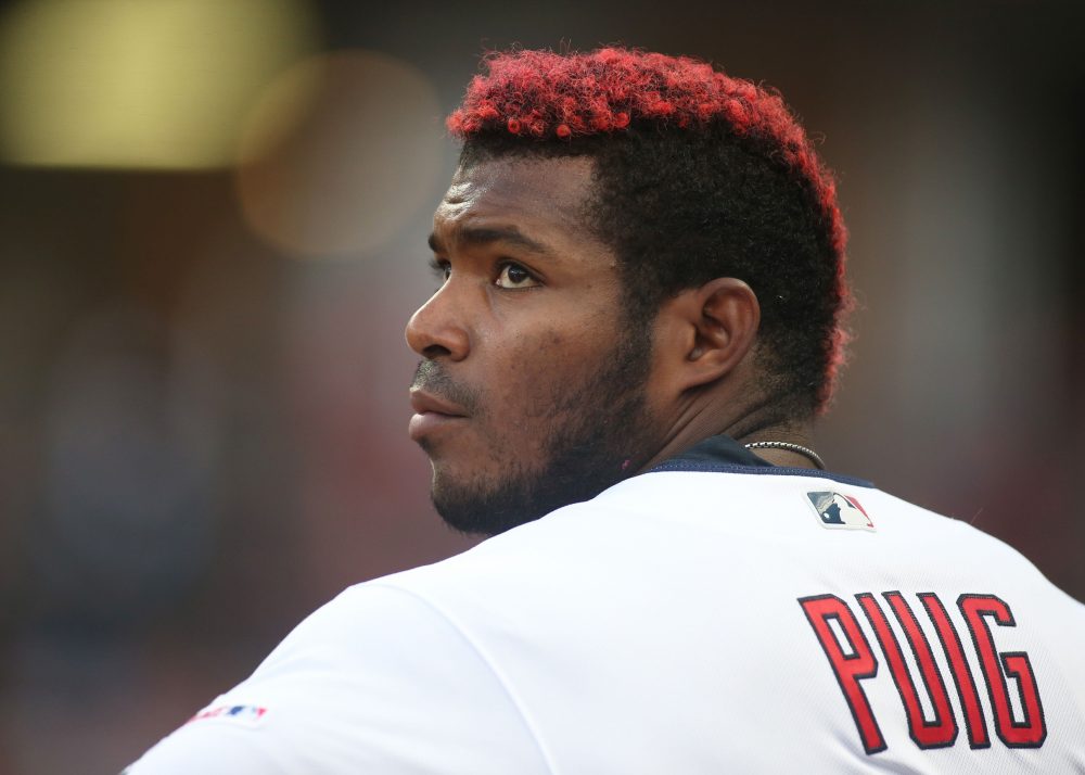
Why do we care though? Let’s put it in the form of an example. Say you’re a GM in February 2018. You get a call from the Dodgers, and they are ready to part with Yasiel Puig on the last year of his contract. In exchange, they’re looking to pull three prospects from you. The consensus is that over the lifetime of the trade, you’d expect to make out slightly better in the long run with team control of the prospects than you will with one year of Puig. But at the same time, you can see that your window is closing, and a 3.0 WAR 2018 season from Puig should bounce your projected record from a chance at a wild card slot to a pennant contender. Puig would be going into his age-27 season in 2018, and in the previous season, he had 3.8 WAR. Do you take the trade?

Ultimately, what any GM would want in this situation is a prediction of the likelihood that Yasiel Puig gives a 3.0 WAR season in 2018. Do we have a 80 percent chance of making the target numbers? One-in-four? Five percent? This is a capability that hasn’t appeared in the public baseball literature to date—and one that we could learn a lot from.

The delta method, k-nearest neighbors, and player aging

Thus begins the quest: we want to describe the process of player aging in terms of the probability of any given outcome, rather than just a single predicted outcome. To understand how this departs from the status quo, we start with the two primary ways that we currently think about player aging. The first is called the delta method which describes the average change between all of the age-n seasons and the corresponding age-(n + 1) seasons.

The delta method is used to describe the mean aging curve, across all or some subset of major league players, simply by looking at the mean of all of the transitions from age-n to age-(n + 1) seasons. You can read about the delta method and its derivatives all over the baseball internet.  Do so, and you’ll find one thing in particular: No one ever uses it to predict individual player performance, only the general trend of the “average player”. We can pretty easily see why this is with a single graph.

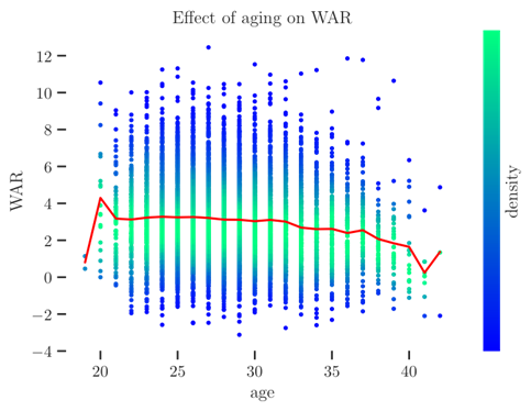
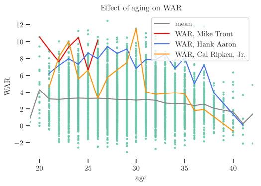
The plot above shows every player season since baseball was properly integrated as a dot, and colored by the density of points in the vicinity of the mean, where many dots overlap. Meanwhile, the average across all of these players is shown with the red line. From this plot it’s very clear that the mean behavior—the subject of the delta method—and the season realized by any given player are not necessarily in the same vicinity. We can also augment this plot by overlaying trajectories of some no-doubt hall-of-famers:

and of some players who have made perfectly servicible contributions over their careers:

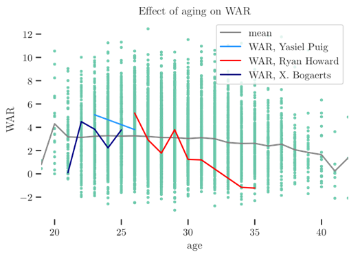
It’s very clear that the predicted average change from an age-n season to and age-(n + 1) season is going to struggle to describe, for instance, Mike Trout’s career trajectory. Put another way, the changes in WAR for the average player- less than 0.5 WAR for any given age-n to age-(n+ 1) season are going to account for very little of the real decay of high-value and even modestly-above-average players, who are often the players we most want to be able to project. The delta method is informative, but not a realistic path forward for understanding how any given player will age.

When it comes to predicting the aging of particular players, a common method is known as k-nearest neighbors. There is literature that can be found that explains how it works and applies it to baseball problems. There are two things I want to point to when it comes to k-nearest neighbors. One is North Korea. North Korea is immediately sandwiched between China and South Korea, and its next two nearest neighbors geographically are Japan and Russia. None of these countries are particularly undeveloped, and its two nearest neighbors are extremely developed. Of course, there are a lot of other variables, on which North Korea is very far from its geographic neighbors: GDP, trade tendencies, and civic and economic structure, to name a few, and it turns out that most of these are more important to the outcome of development than geographic location. So too with baseball: k-nearest neighbors depends on a good choice of variables to describe the “distance” of interest, and they must be good indicators of the thing you’re ultimately interested in. Doing so is a much more complicated task than meets the eye.

Second, k-nearest neighbors will typically only gives a small sample: rarely enough to describe the probability of a given WAR in the next season. This is true even assuming that you could define a perfect distance measure for measuring the similarity between two players and thus allowing you to predict a player’s WAR from one year to the next using k-nearest neighbors. This isn’t to say that the method isn’t useful: it’s just to say that there is room for improvement, and there is room for innovation in defining probabilistic aging predictions for real players. In fact, using the results to follow as a prior distribution for Bayesian k-nearest neighbors analysis may in fact prove to be a means of getting a probabilistic guess of a player’s future value. Nonetheless, this only further cements the potential usefulness for a probabilistic player aging model.

Going probabilistic

My goal, at the end of the day, is to squeeze more of an idea how aging works from the same data that is used to generate the traditional aging curve, which is to say that I want to extract more from a table whose columns contain the WAR for one player from one season, the previous season’s WAR, and the player’s age during those seasons. Now, however, instead of immediately averaging, I want to ex- tract more information from it about how a player will age than just taking the average. In order to understand the interplay between two variables, we can look at the change in WAR for pairs of successive seasons:

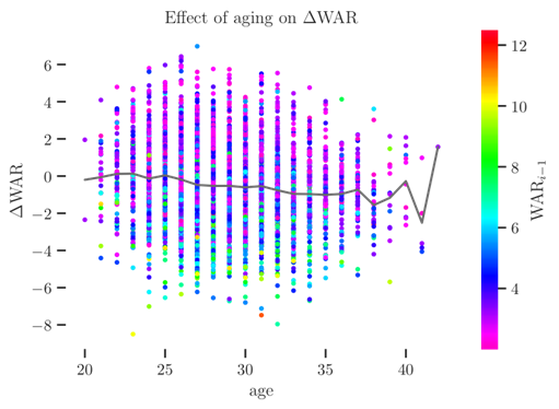
The coloring here is by the first season of the pair represented by a given dot, and what I want to convince you with the plot is that a bad season is more likely to be followed by a significant increase and a good season is more likely to be followed by a significant decrease. In other words, the mean change that is used by delta method to predict is not independent of the season that a player just had.

Luckily, though, if you look at not just the change but the percent change (the change divided by the first season of the pair), we can find a distribution whose mean is significantly decorrelated from skill of the player:

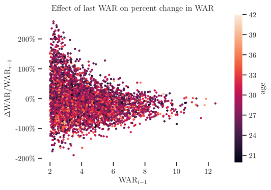
It’s not perfect decorrelation by any means, but we can see that a player is likely, independent of their skill level, to lose on average around 25 percent of their value from one year to the next, but the actual outcomes have a significant spread, which is non-trivially dependent on their skill level. Another glimpse at this data is seen here:

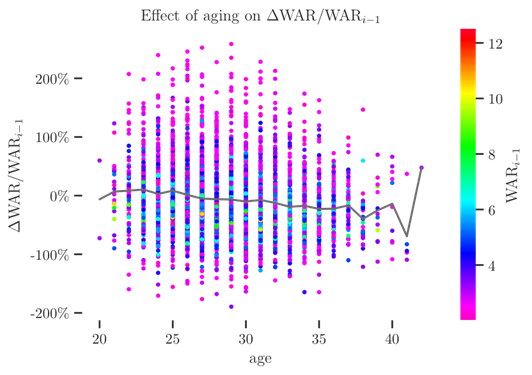
With this plot, it is clear that there is an exploitable pattern: the percent change from one year to the next in WAR follows roughly the same family of distributions, for which the parameters (mean and variance, namely) vary with age and skill level in the first season of a pair.

At this point, I hope it is clear that the current way of doing business leaves something to be desired, and that there is more to be understood and exploited about the probabilities of any given player aging pattern than the previous works on aging have used. In my next post, I’ll develop a method for predicting player aging that will try to take advantage of these observations.