
It is no secret that baseball plays differently in different stadiums. Unlike other sports, baseball sees these differences as a feature, not a bug.
Because stadiums matter, baseball analysts try to account for the effect of differing stadiums. Traditionally, these adjustments take the form of “park factors,” which track and adjust for frequencies of different outcomes at different parks. However, with the advent of Statcast measurements, we have the opportunity to make these assessments more precise. We also want to quantify not only how parks perform on average, but how they vary from day to day.
Today, we introduce the updated family of BP Park Factors. These park factors offer several features:
- They specify the volatility in a park’s day-to-day scoring environment through volatility (a/k/a uncertainty) intervals. This improves modeling accuracy and accounts for the reality that few stadiums offer similar conditions for each game.
- They account for Statcast batted ball inputs, rather than just raw outcomes. This should make them more accurate over shorter periods of time.
- They tend to require fewer seasons of data to work well. BP’s park factors will thus reflect reasonably-current conditions.
Our new park factors are reflected in our PECOTA projections for 2021, giving BP Premium subscribers seamless access to BP’s new park factors and their potential to optimize fantasy teams. The park factors for each player are also applied based on the team’s actual game-by-game schedule, not just a home park factor divided in half.
This release of park factors will cover major league parks over the 2015-2020 seasons; as we settle on a suitable alternative for non-Statcast seasons and non-Statcast leagues, they will be expanded. These park factors will also be posted to BP’s (new) leaderboards in the coming weeks. Premium subscribers who wish to have access to them earlier are welcome to request this data now, as discussed below, and we will provide it.
We also expect these new park factors to be incorporated into DRC+ and DRA- by Opening Day.
Background
Park analysis has been actively conducted for decades. John Choiniere compiled a list of useful resources here. Some of the best work in the area has been generated by Patriot on his Tripod blog.
Generally speaking, park effects are challenging to isolate. In part, this is because baseball is a high-variance sport. But another problem is that park effects are latent, always wrapped within some combination of batter and pitcher performances. Effective park factors must cut through this variance without being tricked by the sample of players that just so happened to play in the park over the time period of interest.
One approach is to use a so-called batting park factor. Instead of estimating a park’s effect directly, this method asks a different, but related question: How do each team’s batters perform at home versus when they are on the road? Because a park’s effects can only be observed through player performance, and because a park’s home team plays there the most, we can leverage this and treat teams’ ratios of home and away runs scored as a (partial) reflection of how home parks differ.
Another approach is to focus on the performance of visiting teams, making additional adjustments for quality of competition and other factors. (For example, a team cannot face its own pitchers). This, however, throws out half of the data (always undesirable) and considers only teams that are already experiencing an additional, “away from home” penalty. Sequential adjustments also risk a “ping-pong” effect from continued, mean-reverting over-corrections, which can be exacerbated when much of the data is being disregarded from the start.
Both methods can be noisy in small samples, so analysts frequently combine multiple recent seasons (typically three, but sometimes more). This can improve accuracy, but by smoothing over multiple seasons, multi-year park factors risk removing much of what is interesting about parks: their year-to-year, and even within-season variation.
Ideally, we could target these challenges instead through a well-specified regression. Regression allows us to consider both home- and away-team performances. Regression also allows us to use all of the data, make desired adjustments simultaneously, and it doesn’t limit us to ratios of home versus away team scoring. Preferably, we would maximize regression accuracy by using not only more information, but better information.
Updated, Statcast-based Park Factors
Since 2015, MLB’s Statcast system has tracked various qualities of batted balls, and has done so in increasingly accurate fashion. How do we best benefit from this new information?
One option would be to rely upon an existing Statcast-based metric, like expected weighted on base average (xwOBA). For example, one could look at the difference between xwOBA and regular weighted on base average (wOBA) on balls in play and assume that any differences are caused by the park where the game is played. E.J. Fagan explained how such a system might work. Alex Chamberlain has studied the issue as well; Eno Sarris and Dan Richards have tried to achieve similar results from other Statcast-derived metrics.
However, there are also reasons not to take this approach. The greatest concern is that this would tie our park factors to the output of a third-party metric, for better or worse. It could also exclude important additional information, such as the horizontal directionality of the ball, which xwOBA and its derivative metrics like Barrels do not consider. We want the benefit of that information, because ballparks can be asymmetric; any metric that relies solely on launch angle and exit velocity (a/k/a “launch speed”) implicitly assumes the exact opposite. Finally, treating all differences between xwOBA and wOBA — or between any expected metric and actual results — as caused solely by stadium conditions is a sweeping assumption. We think it wise to be a bit more skeptical.
So, in creating our own system of updated park factors, we opted to use semiparametric binomial regression. Specifically, we have employed hierarchical generalized additive models (HGAMs), one each for home runs, triples, doubles, and singles, with the denominator always being outs. The home runs version of this model is specified in R as follows:
##### Load Package #####

library(mgcv)
library(tidyverse)

##### Run Model #####

HR.mod <- gam(home_run ~
                s(launch_speed, launch_angle, k=60) +
                s(gameday_x_coord, k=15) +
                temperature +
                s(stadium_batter_side, bs="re"),
              data=BIP, family="binomial",
              method="REML")

##### Extract and Marginalize #####

BIP.preds <- BIP

### the actual predicted outcome ###

BIP.preds$HR_all <- predict(
  HR.mod, type='response')

### marginalize over park and temperature ###

BIP.preds$HR_no_park <- predict(
  HR.mod, type='response',
  newdata = BIP.preds %>%
     dplyr::mutate(temperature = mean(BIP.preds$temperature),
  exclude = c("s(stadium_batter_side)"))
The predictors we use fall into three primary categories:
- Batted ball measurements: For each ball put into play, we specify splines with varying combinations of launch speed, launch angle (first converted to radians), and horizontal fielding location, all centered and scaled toward the unit interval. The first two values are publicly-available Statcast measurements of the baseball right off the bat. Because the ball’s horizontal “bearing” is not published, we instead use the venerable Gameday “x” coordinate, by which stringers estimate a ball’s “fielded” location. It offers a surprising amount of useful information in its own right. We use thin-plate regression splines, which are accurate and efficient, and we specify them from one to three dimensions, depending on the batted ball type in question, to incorporate all these measurements.
- Temperature: Second, for home runs only, we account for initial game-time temperature. Temperature has a clear and consistent effect on the distance that a baseball will travel when struck. Temperature does not fully reflect all playing conditions at the stadium, and temperatures can change over the course of a game, but game-time temperature still tells an important story. Temperature does not seem to materially affect other hit types.
- Modeled groups: Finally, we add a so-called random effect to track batter-handedness (a/k/a “batter side”) on balls struck within these parks (“stadium_batter_side”). This variable recognizes that batter-handedness tends to affect where batters hit the ball, allowing us to track stadiums which on average play differently for right-handed batters than for left-handed batters. This is not as precise as modeling specific stadium dimensions, but it summarizes them in a way that traditionally has proved useful, as we can map stadium characteristics to obvious hitter traits. It also incorporates the skepticism mentioned above: through shrinkage, we credit parks for their results not otherwise explained by other measurements, but only after they persistently demonstrate a certain trend.
For the purposes of our home run park factor, note that we “credit” stadiums with the effect of their game-time temperatures, here by predicting off the grand mean of all game-time temperatures. Traditional park factors implicitly do this anyway; we make it explicit because temperature is a factor, extrinsic to participant skill, that varies by park and is part of the net effect a park’s location has (or does not have) on batted balls.
Keeping with tradition, we will report park factors on the traditional “100” scale, where 100 is average, a higher value indicates batter-friendliness, and a lower value indicates pitcher-friendliness. Park factors will be offered both by batted-ball component (“component park factor”) and by the overall effect on run production for all such components combined (“run park factor”). Our park factors, as expressed on the 100 scale, are always multiplicative of the league average rate for the component in question.
The Importance of Park Volatility
As noted above, our new park factors introduce a new feature: Park Volatility, as represented by the “upper” and “lower” values for each park’s effect. This volatility will be captured by volatility intervals, generated by a Bayesian bootstrap on the models’ predicted results. A simplified, but illustrative version of the R code for the bootstrap is as follows:
### Load Packages #####

library(doFuture)
library(future.apply)
library(tidyverse)

##### Perform Bayesian Bootstrap of average differences #####

stadium.draws <- future_lapply(
  seq_along(1:5e3),
  function(x){

    stadium.tmp <- BIP.preds %>%
      dplyr::mutate(

### generate random positive weights ###
        exp_rand = rexp(nrow(BIP.preds), 1),
### normalize to a Dirichlet distribution ###
        samp_weights = exp_rand / sum(exp_rand)) %>%
### sample from the Dirichlet, with replacement ###
      dplyr::slice_sample(., prop = 1,
                          weight_by=samp_weights,
                          replace=TRUE) %>%
      dplyr::group_by(stadium, batter_side) %>%
      dplyr::summarise(
       HR_stadium_eff = mean(HR_all - HR_no_stadium)
      ) %>%
      dplyr::ungroup() %>%
      dplyr::arrange(stadium, batter_side)

    list(
      HR_stadium_draw = stadium.tmp$HR_stadium_eff
    )

  }, future.seed = 1234)

##### Extract all draws of HR park factor distribution #####

HR_stadium_dist <- simplify2array(lapply(stadium.draws, function(t) t$HR_stadium_draw))
The desired summary or quantile statistics can be extracted from there.
For advanced users who incorporate our park factors into further models, using these volatilities while inserting our park factors will achieve even greater accuracy than using the raw average values. This works better for the same reason that random sampling of imputed variables works usually better than imputing mean values: the variance of the predictor is a core part of its relationship with the outcome, and you lose that if you plunk the same value down for every row.
Uncertainty is important in all models, because without it you have no idea whether the differences between the numbers you generate are meaningful. With park factors, though, uncertainty can be critically important. This is because the calling card of many parks is not just whether they are, on average, favorable to batters or pitchers, but rather how volatile they are from day to day. Trying to summarize the seasonal conditions at Wrigley Field with a single, average value is tough to do. By tracking the uncertainty around our estimates, BP’s Park Factors thus quantify both the average park factor and the volatility around that average value.
To illustrate why this matters, consider the following plots of BP’s home run park factors for certain (1) above-average stadiums and (2) below-average stadiums over the 2019 season. The solid dots indicate the average park factor for each park / batter-side, and the horizontal bars show the volatility around those park factors. Again, 100 is average. To declutter things, we have selected only a few stadiums in each group.

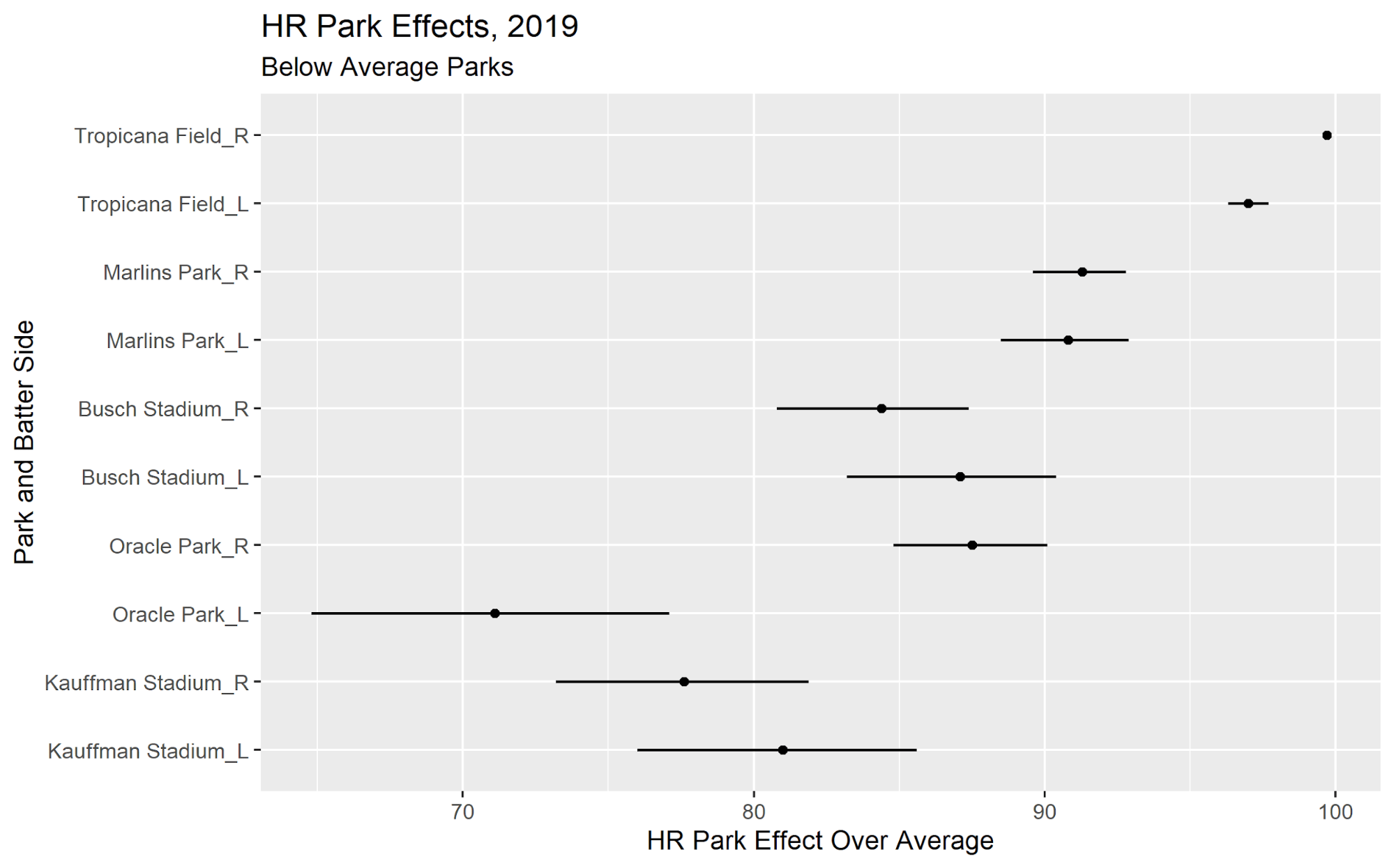
The overall ordering of the stadiums may not surprise you much (aside from the fact that Dodger Stadium can be a great place to hit home runs: it is, particularly for right-handed hitters). But check out the volatility! Some parks have fairly tight distributions from day to day whereas others have much wider distributions. The most sensible explanation is that this volatility reflects weather and other changes in playing conditions at the stadium. This conclusion follows from the fact that Tropicana Field, a dome environment, has essentially no volatility range at all, whereas stadiums like Great American Ball Park (a known launching pad on certain days) and Oracle Park (here comes the fog!) tend to have much wider ranges.
This is why it is beneficial to sample from a distribution of a stadium’s park effect instead of using the same value for every game. By using only an average value —which is the traditional practice — you pretend that park conditions are exactly the same every day, which is obviously not true (Tropicana Field possibly excluded). Without random sampling, readers will end up attributing blame (or credit) to players that do not deserve it, and will not maximize the return on these park factors. Incorporating this volatility into one’s personal projections is not a trivial process, but for those willing to take the plunge, it could be an exciting opportunity.
Accuracy
We illustrate the accuracy of our new park factors by investigating their ability to explain actual production of various batting events, over different combinations of years. This is useful because park factors have at least three distinct applications: (1) to project entirely future performance; (2) to track in-progress performance during an active season; and (3) to help explain past performance once a season has concluded. The traditional practice of combining multiple previous years of park performance offers essentially the same answer to all three questions. We prefer to validate the use of fewer years, and ideally use a single year of park factor data, to allow parks to exhibit reasonable annual variation. This also allows us to offer separate answers to each of these three questions.
For this exercise, we randomly sampled 50,000 batted balls from each of the 2016 through 2020 seasons, which is about half of a typical season (this helps keep our training data at a manageable size). We then ran and evaluated how well our component models explained the results of our target seasons, which were 2018, 2019, and 2020. We tested three target seasons and averaged the results so that one season could not affect our results too much. We then resampled the predictions 5,000 times using a Bayesian bootstrap to derive the overall averages and the uncertainties of these estimates over those three seasons. Finally, as a baseline we selected 50,000 random batted balls from all across MLB over the previous three seasons to test the contrary hypothesis that all parks are essentially the same, give or take some variance.
Here are the results:
Home Runs
| Predictors of Target Season | MAE | MAE SD |
| League-wide sample, 3 previous seasons | 0.286 | 0.002 |
| 3 previous seasons | 0.110 | 0.001 |
| 2 previous seasons | 0.110 | 0.001 |
| 2 previous seasons + current | 0.094 | 0.001 |
| 1 previous season + current | 0.094 | 0.001 |
| Previous Season | 0.107 | 0.001 |
| Current Season | 0.094 | 0.001 |
The first column indicates the predictors used for our target season; sometimes the predictors included the target season’s data and sometimes they did not. As noted above, depending on your objective, you sometimes have the target season’s data available and sometimes you do not. The scoring metric (second column) is the mean absolute error (MAE) off the actual results and the SD in the third column is the uncertainty above or below our MAE over all our draws. Lower MAE is better. Differences between measurements are more likely to be meaningful if they exceed the SDs around their respective values (often described as the “plus or minus” or “margin of error”).
These tests show that a single-season park factor (“Current Season”) works just fine for retrospective work, and that a running combination of the previous and current year should work equally well for season-in-progress estimation. For pure projection purposes, it is sufficient to use the previous season’s park factor to project the following one: adding more previous seasons of data makes the park factor less accurate, not more so. And finally, the information added by these park factors is much, much better than a random sample from across the league, confirming that their value is no mirage.
We of course prefer single-year park factors, and at least for home runs, this analysis validates that choice. There no longer appears to be any need to smooth over three, four, or five previous years. We can now capture the oddities of each park over each season without sacrificing overall accuracy.
Triples
| Predictors of Target Season | MAE | MAE SD |
| Random sample of 3 previous seasons | 0.042 | 0.001 |
| 3 previous seasons | 0.052 | 0.001 |
| 2 previous seasons | 0.051 | 0.001 |
| 2 previous seasons + current | 0.040 | 0.001 |
| 1 previous season + current | 0.040 | 0.001 |
| Previous Season | 0.047 | 0.001 |
| Current Season | 0.040 | 0.001 |
No way around it: triples are more challenging. In part because of their rarity, triples are difficult to predict with consistency.
Here, our single-season park factor again performs best, tied with our in-season use of current and the previous year. Troublingly, the accuracy becomes no better and arguably worse than a random league-wide sample as more seasons are added. Projecting triples remains quite difficult, although in fairness, we made no effort to optimize our models to account for multiple years of data. But at least we know we offer some value both during and after the season of interest.
Doubles
| Predictors of Target Season | MAE | MAE SD |
| Random sample of 3 previous seasons | 0.409 | 0.003 |
| 3 previous seasons | 0.273 | 0.002 |
| 2 previous seasons | 0.271 | 0.002 |
| 2 previous seasons + current | 0.263 | 0.002 |
| 1 previous season + current | 0.263 | 0.002 |
| Previous Season | 0.273 | 0.002 |
| Current Season | 0.262 | 0.002 |
Fortunately, with doubles we are back on the wagon again.
The retrospective, single-season park factor again performs best, and the combination of last season and current season provides essentially identical in-season performance. Accuracy drops slightly as we move toward using previous seasons only, but notably, adding more seasons does not seem to help much. The previous year’s park factor is once again sufficient for projection purposes. All of these park factor estimates are far better than a random sample from across the league.
Singles
| Predictors of Target Season | MAE | MAE SD |
| Random sample of 3 previous seasons | 1.051 | 0.004 |
| 3 previous seasons | 0.561 | 0.002 |
| 2 previous seasons | 0.562 | 0.002 |
| 2 previous seasons + current | 0.565 | 0.002 |
| 1 previous season + current | 0.566 | 0.002 |
| Previous Season | 0.578 | 0.002 |
| Current Season | 0.567 | 0.002 |
Singles again show strong overall performance, far better than random league average. Perhaps due to the volume and general dispersion of singles, all of the seasonal combinations perform somewhat similarly. Singles are the one hit type for which you could justify using multiple previous years, and perhaps only those previous years at all times. The differences are sufficiently small that we feel comfortable once again using a single-year park factor for retrospective analysis and also the current-plus-one-past-season combination for in-season work. But it is possible that a more backward-looking analysis could perform slightly better.
Between the recent changes in baseball composition and the bizarreness of the 2020 season, all of these patterns merit ongoing, at least annual review.
Run Park Factors
Although component park factors are interesting, the number that often interests readers most is the park’s “run” factor: taking all of these components together, and recognizing that some events (like home runs) are much more valuable than others (such as singles), what is the overall scoring environment at a given park for the season?
According to our analysis, here are the top and bottom run park factors for stadiums by batter side in 2020. The “lower” and “upper” bound values provide the 95th percentile Volatility Interval around the average park run factor, or “PF”:
Top Park Run Factors
| Season | Park | Batter Side | Run_PF | Lower Bound | Upper Bound |
| 2020 | Fenway Park | R | 109.5 | 107.9 | 111.1 |
| 2020 | Great American Ball Park | R | 108.2 | 105 | 111.9 |
| 2020 | Great American Ball Park | L | 107.9 | 104.7 | 111.6 |
| 2020 | Fenway Park | L | 107.3 | 105.4 | 109.4 |
| 2020 | Citi Field | L | 106 | 104.5 | 107.7 |
| 2020 | Coors Field | R | 105.3 | 104.2 | 106.6 |
| 2020 | Coors Field | L | 105.2 | 103.2 | 107.4 |
| 2020 | Citizens Bank Park | L | 104.7 | 103.2 | 106.3 |
| 2020 | Dodger Stadium | R | 104.6 | 102.1 | 107.5 |
| 2020 | Sahlen Field | L | 104.3 | 102.6 | 106.2 |
Bottom Park Run Factors
| Season | Park | Batter Side | Run_PF | Lower Bound | Upper Bound |
| 2020 | Guaranteed Rate Field | L | 97.4 | 95.5 | 99.2 |
| 2020 | Target Field | R | 97.2 | 96 | 98.2 |
| 2020 | Yankee Stadium | L | 97.2 | 96 | 98.7 |
| 2020 | Oakland Coliseum | L | 97 | 95.1 | 98.7 |
| 2020 | Comerica Park | R | 96.4 | 95.1 | 97.7 |
| 2020 | Busch Stadium | R | 96.1 | 94.6 | 97.5 |
| 2020 | Oakland Coliseum | R | 96 | 94.7 | 97.2 |
| 2020 | Dodger Stadium | L | 94.7 | 93.1 | 96.4 |
| 2020 | Petco Park | L | 93.7 | 92.3 | 94.9 |
| 2020 | Busch Stadium | L | 93.6 | 91.5 | 95.4 |
Conclusion
We are excited by our updated park factors, and we welcome your feedback, politely-phrased questions, and suggestions.
We caution that there is still likely room for improvement: we have made choices that favor interpretability and computational speed. Our goal was to bring our park factors into the modern age, not to pretend there is only one way to model park factors effectively. More aggressive modeling options are available, such as those discussed in this terrific paper, but it is unclear how practical they are for large data sets or for park factors more generally. We also still need to decide how to model non-batted-ball park factors (if we elect to model them at all) and non-Statcast ballparks and seasons. We expect decisions on these in the not-so-distant future.
BP Premium Subscribers who wish to get the complete set of these park factors now should email our customer service team at cs@baseballprospectus.com, to receive a comprehensive spreadsheet for their personal use. The spreadsheet will include breakdowns of these components that make it easier to perform the distributional sampling that I described above. For the general public, we expect that our new park factors will be posted on our new leaderboards when they are released over the next few weeks.
Thank you for reading
This is a free article. If you enjoyed it, consider subscribing to Baseball Prospectus. Subscriptions support ongoing public baseball research and analysis in an increasingly proprietary environment.
Subscribe now