
Player aging is a key issue in the projection of player performance. Effective aging analysis is worth literally millions of dollars to professional sports teams and considerably less but still material sums for players of fantasy sports games.
The “delta method” has become a popular method to measure player aging.[1] Often credited to Tom Tango and Mitchel Lichtman in baseball, it has since been extended to hockey and other sports. CJ Turtoro gives a detailed history of multiple studies by analysts in baseball and other sports. I strongly recommend his write-up and the links he provides.
However, not everyone agrees that the delta method is the way to go. Several others, primarily in the academic community, have instead used parametric regression models, using a different data structure than the delta method. The most famous of these efforts may have been that of JC Bradbury. Bradbury famously claimed in 2009 that performance for most baseball metrics peaks at a baseball age of 29, while adherents of the delta method, especially Lichtman, have insisted that players tend to peak at much earlier ages. This dispute led to quite the online donnybrook.
These Aging Wars have aged a decade themselves, and it is past time to reevaluate the delta method and possible alternatives. Using out-of-sample performance as our guide, we find that semiparametric regression using a more traditional, “across player” data structure may be just as good, and possibly superior to the delta method in evaluating the aging of hitters. It also involves less work. We further find that neither Dr. Bradbury’s method nor the delta method may accurately diagnose the true “peak age” of average baseball hitters, although the practical effect of this is probably minimal.
Measuring Batting Contributions
We evaluate the accuracy of the delta method through its ability to estimate the aging curve for the batting statistic On-Base-Plus-Slugging (OPS). OPS is somewhat inelegant in design, but it effectively represents batter run contributions, at least in the aggregate.
For ease of understanding, we convert each player’s OPS for each season to an OPS above or below the average MLB OPS for that season. This would mean the average OPS above average is zero, with good seasons having positive values and below-average seasons negative values. This adjustment helps control for changes in the offensive environment, should be easier to understand, and provides the additional benefit of showing how each age group performs relative to overall league average rather than only peak age, as is typical for many studies.
To train our methods, we will use all position-player baseball seasons in MLB from 1977 through 2016. We chose these years because they are what Lichtman used for his most recent, 2016 study, and because they allow us to set aside the 2017–2019 seasons for testing. Like Lichtman, we also use only ages 21 through 41. To ensure a clean break, we will only use batters whose careers started after 1976. We round baseball ages to the nearest integer age.
The Delta Method
The delta method is a non-parametric, arithmetic approach that proceeds as follows:
- Restructure a dataset of player seasons around back-to-back seasonal performances (“seasonal pairs”) for all players who have had back-to-back seasons in major league baseball.
- Throw out the rest of the data (all player seasons without a following player-season).
- Calculate the weighted average of all player performance changes (i.e., “deltas”) for each baseball age, weighted by the player’s participation level (typically plate appearances for batters) over both seasons. (Lichtman currently seems to prefer the harmonic mean).
- “Chain” these average deltas for each age to form an overall curve (time series, really) of the various gains and losses of average ability by age.
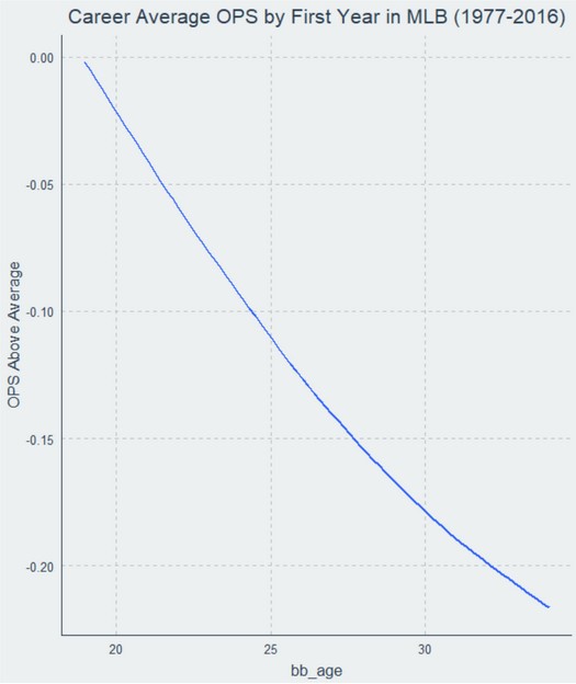
If we do this for all seasonal pairs in the dataset, we end up with the following curve:
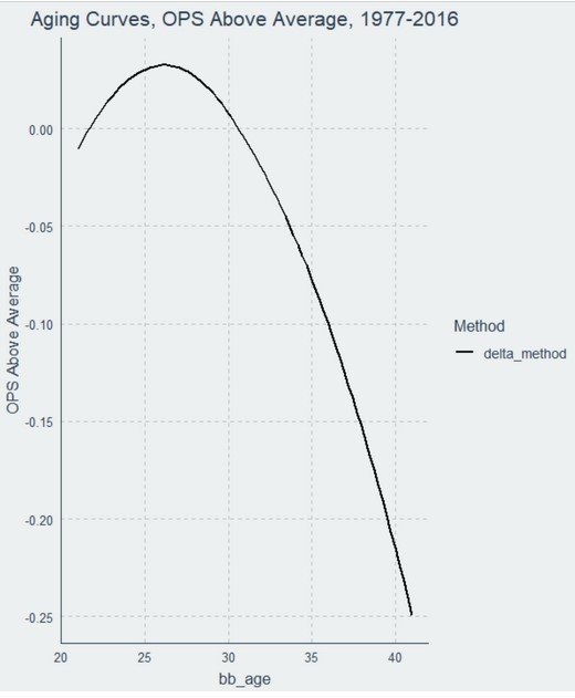
The delta method is somewhat intuitive: if you want to know how the performance of athletes changes as they age, then look at all changes in performance that occurred in consecutive seasons for these athletes and average those changes by age across all players.
However, the requirement of consecutive seasons can also be problematic. Under the “seasonal pairs” structure of the delta method, all player seasons without an adjoining season are discarded. Every final year of any player’s career is effectively discarded. Players who appeared for only one season are discarded. Players younger than 21 may not be considered because there is not enough consecutive-season data. Ditto for the oldest players in the dataset. In sum, over 20 percent of the data—several thousand seasons—gets thrown out. That’s a concerning number, particularly if you want to focus on these or other subgroups.
I also strongly recommend a fifth step if you plan to apply the delta method, and that is to re-center the chained results at the average age of the chained values, weighted by plate appearance volume. I have not seen other analysts discuss this, but failing to do so will result in worse predictive performance, because everything ends up being measured relative to player performance at 21 (or wherever your chain starts) instead of the average age in baseball. The effect of this recentering is an improvement of about 10 points of OPS in predictive accuracy. Giving the delta method this considerable benefit of the doubt, we will center the chain for our analysis here.
After recentering, which is already reflected in the plot above, the delta method says that the youngest batters tend to hit below league average at first, then quickly improve to above league average as they age. The peak age for OPS according to the delta method in this dataset is 26. After that point, players begin a rapid descent, losing almost 300 points (!) of OPS between their peak age and age 41.
The “Survivor” Correction to the Delta Method
In addition to the delta method, we will consider what Lichtman calls a “survivor bias” correction. Lichtman proposed this correction in 2016 as an improvement on his previous efforts.
The asserted basis for the correction is that players who are randomly unlucky in their last season may not return in the following season, whereas those who were fortunate will return and on average play more poorly. This, Lichtman hypothesizes, could cause the delta method to overestimate aging effects. This strikes me as being more about theoretical bad luck than true survival bias, but it functions as a “correction” nonetheless.[2]
The procedure Lichtman describes is somewhat involved, and the exact code is not provided. But Lichtman describes (and plots) the result as an average rise of eight points of weighted on base average (wOBA) (~20 points of OPS) up to age 26/27, and then an average decline of three points of wOBA (~8 points of OPS) from ages 28 onward, so we will use that as our approximation, and index the peak of this corrected curve to the peak of the delta method so they are on the same average scale.
Here is what the “corrected” curve looks like compared to the original delta curve:
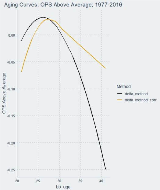
This curve looks more reasonable, at least in some respects. It has young players starting well below average, rising above league average around 25, still peaking at age 26, and then declining much more gradually until age 41, when players end up a little over 60 points below league average. It allows for a total aging effect of 99 points of OPS over the course of a player’s career.
A Semiparametric Alternative
Third, to reflect current standard practice for non-linear models, we consider a general additive model (GAM). In this model, we regress OPS above average on a thin plate regression spline for baseball age, and further control for each player’s career average performance as an alternative to using seasonal pairs. For simplicity, Gaussian errors (the default) are assumed. This requires no reorganization or disposal of any data. It does require first calculating each player’s career mean OPS above or below MLB average.[3]
We label this a “GAM Across” model, because it is a GAM calculated “across” all player seasons (the natural state of the data) and does not require reorganized “seasonal pairs.” This GAM is not the best we can do, but it is representative of how a knowledgeable analyst might begin to tackle the problem in this day and age, starting from scratch.
Here is how the GAM Across aging curve compares to the two delta curves:
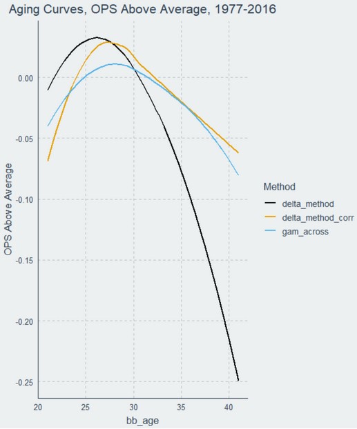
The GAM Across curve is much more gradual than the other two. The GAM Across model finds that players in this dataset tend to perform below league average until about age 25, then peak around age 27. The average player then gradually declines, falling below league average by 32 and declining more rapidly thereafter. Like the corrected delta method, the slopes of the ascent and descent are different. The entire range of aging effects spans 95 points of OPS.
We will also discuss other models below, but these will be our three primary choices.
Testing the Aging Methods
Most work justifying aging methods appears to be theoretical in nature, with Turtoro’s analysis a notable exception. Because the vast majority of people using aging curves do so for the explicit purpose of explaining performance, though, the better way to evaluate an aging method is to test how it actually works in practice.
But how do we do this? Traditionally, we test different models by seeing how well the methods generalize; in other words, how well they measure data they have never seen before. This increases the likelihood that a model is describing an underlying process rather than just the sample of data it happened to receive for analysis. We can test for generalizability in a few different ways:
- We could use cross-validation: split all of our data into portions and sequentially train and test the models on each combination of training and testing data, and take the average error over all combinations.
- We could resample the data with replacement (e.g., bootstrap), and take the average error over all of those combinations. If done enough times, bootstrapping is arguably more efficient than cross-validation.
- We could hold out certain years entirely from our datasets and use them for testing only, measuring the error in what each model predicts versus the true results from those seasons.
- We could combine some of these concepts by randomly reshuffling the data to hold out different seasons, and take the average error of the methods’ attempts to explain each of the held out combinations.
All of these concepts have value and some of them can be combined. We’ve decided to test our three aging methods in two ways.
First, because we train our data only on years 1977 through 2016, that leaves 2017 through 2019 as “held out data” which we can use to test the methods’ ability to diagnose actual trends, and forecast the consequences of those diagnoses. With only three seasons of data to test, the standard errors will be large, but there is definite value in being able to explain what literally did happen in later seasons. Forecasting the future is the primary reason people use aging curves, so there is no good excuse for being any worse at it than necessary.
Second, we want to ensure that our methods are good not only at predicting seasons, but also at predicting careers. We can evaluate this through what I call “leave career out” resampling: randomly select several hundred careers, hold them out, train each method on the remaining careers, and average the error in estimating the effect of age on the held out careers over several resamples. We elected here to randomly hold out 625 careers at a time (roughly, the number of different position player batters in a modern MLB season), and repeat this procedure 5,000 times until we were satisfied the values had converged. This amounts to roughly an 80-20 split of training to testing data on each resample.
Some might argue that “leave-career-out” cross-validation reflects a biased sample of “surviving” players, or is inferior to simulating hypothetical careers. While this is possible, I think the proposed tests still have great value, for the following reasons.
First, while I welcome any reasonable alternative, constructing simulated careers begs the question of the basis for those simulations. The best empirical evidence we have of future careers is the set of careers we have already seen. And through resampling, we are effectively conducting a series of de facto simulations.
Second, although we cannot usually account for hypothetical seasons from players who dropped out of baseball, we have seen plenty of seasons from players who remained in baseball years beyond what their hitting prowess alone would have justified. This is particularly true at premium defensive positions. The resampling process ensures that we will see plenty of these hitters over the various samples, and some samples should randomly include a disproportionate number of them. These hitters should help represent theoretical batting seasons from players who dropped out but still have useful aging information to contribute.
Third, regardless of whether there are additional, hypothetical seasons that would be nice to consider, there is no defensible scoring method that would not also require excellent performance explaining players who actually played. Imagine, for example, telling your baseball GM that while you were doing a second-rate job estimating actual players, she should take heart in the fact that you can nail the theoretically-justified, invisible players. (If you actually tell her this, please ensure your LinkedIn profile is up to date).
So, recognizing that no scoring method is perfect, we will test these aging methods on two criteria: (1) the ability to predict, using only 1977 through 2016 seasons, the performance of players by age during the 2017 through 2019 seasons; (2) the ability to predict, over 5000 resamples, every meaningful combination of held-out player careers from 1977 through 2016 who might be playing together at one time.
Of course, if you can suggest a better method, you are welcome to give it a try. We are providing the R code for this article so you can replicate these simulations, tweak the settings, and report back to the community on your findings.
Testing Results
Predicting Effect of Age during the 2017-2019 Seasons
Rated by Mean Absolute Error (I’ve become convinced it is more useful than Root Mean Squared Error), here are the results:
Table 1: Mean Absolute Error, 2017-2019 seasons, OPS as Explained by Age Alone
| Train Years | Test Years | Age Range | Delta Method | Corr. Delta Method | GAM Across Method |
| 1977–2016 | 2017–2019 | All | 0.089 | 0.085 | 0.084 |
| 1977–2016 | 2017–2019 | 21–25 | 0.078 | 0.076 | 0.076 |
| 1977–2016 | 2017–2019 | 26–30 | 0.089 | 0.089 | 0.088 |
| 1977–2016 | 2017–2019 | 31–35 | 0.087 | 0.080 | 0.080 |
| 1977–2016 | 2017–2019 | 36–41 | 0.136 | 0.085 | 0.085 |
The first row lists aggregate performance across all age groups: the remaining rows break down performance within the four subgroups that comprise the whole. Lower error rates are better. Bolded values are the best for each group.
The methods perform similarly in many respects. However, the GAM Across method,[4] using all of the data and not requiring seasonal pairs, does the best job of explaining the effect of age both overall and within selected age groups of the 2017 through 2019 MLB player seasons.
The corrected delta method is an improvement overall on the delta method, is a huge improvement in the 36–41 age group, and is somewhat less of an improvement in the 31–35 age group. Interestingly, the corrected delta method may perform worse than the delta method for players between 26 and 30, the peak range for player performance in this dataset, although the difference is very small.
The delta method is beaten by at least one of the other two methods, and sometimes both, in every measurement.
Again, we are only talking about three seasons and in theory these values are very noisy. However, reality, particularly the most recent versions of reality, “counts” in a way simulations never can.
Predicting Effect of Age on Randomly-Sampled Careers
Our second test considers the possibility that there is some randomness in the distribution of which players happen to be playing major-league baseball at a given time. Therefore, our “leave-career-out” test evaluates different combinations of player careers.
As noted above, we selected 625 careers, fit each aging method to the remaining 2000+ careers, test how well the 625 careers we held out are explained by each method, and then repeat the process 5,000 times and take the average error over all these resampled datasets.
Table 2: Mean Absolute Error, Random Career Combinations, OPS as Explained by Age
| Seasons | Sims | Age Range | Delta Method | Corr. Delta Method | GAM Across Method |
| 1977–2016 | 5000 | All | 0.096 | 0.090 | 0.089 |
| 1977–2016 | 5000 | 21–25 | 0.096 | 0.093 | 0.091 |
| 1977–2016 | 5000 | 26–30 | 0.089 | 0.090 | 0.088 |
| 1977–2016 | 5000 | 31–35 | 0.094 | 0.088 | 0.088 |
| 1977–2016 | 5000 | 36–41 | 0.153 | 0.095 | 0.095 |
This exercise appears to be more challenging for the aging methods than the “test years” evaluation, but the results are fairly similar. The GAM Across method is as good or better than both delta methods in every respect, although with respect to the corrected delta method, the differences are within the margin of error.
The corrected delta method is once again better than the delta method overall, possibly slightly worse during the player peak years of 26 to 30 years old, and then notably better as aging continues.
Without correction, the standard delta method is consistently inferior, and a bit of a disaster starting at age 36, although the standard errors here grow very large due to the paucity of data.
In sum, the standard delta method seems difficult to recommend. The corrected delta method performs much better, but has some issues and is more complicated. The GAM Across method performs as well or better than the other two options in every respect, and does not require post-hoc corrections or rearrangement of the data in order to work well.
Why does the GAM perform well? Part of it may be the fact that it has more data to work with, because the data is organized in its natural format: across players, not within individual players, and no data is thrown out. More likely is that the delta method, like previous-generation smoothing splines, overfits the data by requiring too many “knots”: here, calculating and enforcing an average value for each and every individual age. A thin-plate regression spline looks more directly at the overall structure of the data and is not beholden to the raw annual averages.
When do baseball hitters peak?
Those of you who lived through the Aging Wars (or lived through a review of the comments posted on those articles) may remember that the primary line in the sand between Team Delta and Team Bradbury was over the typical “peak” age for baseball players. Team Bradbury said it was 29 for most statistics; Team Delta said that it was lower. Team Delta said that Team Bradbury’s finding was biased by his decision to use only players with long careers; Team Bradbury responded that when he loosened the career requirements it made no difference. Team Bradbury also retorted that Team Delta was not using rigorous methods; Team Delta said their methods were good enough to know when players were peaking and when they were not.
I know we are all sick of people “both sides-ing” an issue in our current political environment but . . . it is possible that both sides here were actually incorrect, and that both sides were further incorrect about why the other side was incorrect. This, of course, would be a great way to end up in a dispute incapable of being resolved.
Part of the problem is defining what it means to measure “how players age.” What are we trying to find out? The average performance in baseball or average performance of the average player in baseball? These two concepts are not the same, and the distinction matters. I think the latter is the better choice and also is how I suspect people tend to interpret aging curves.
In his article, Professor Bradbury correctly realized that the goal should be to predict how the average player will age. However, he estimates a peak age for OPS—and many other statistics—that is probably too high. Contrary to the suspicions of Team Delta, it probably has little to do with the sample of players Bradbury used. The function provided in the R code for this article allows you to build an “across player” dataset, which Bradbury also appears to have used, with your choice of minimum player seasons. Whether you use players with 1, 5, or 10 seasons of experience, the peak age for batter OPS is still 29. Bradbury was correct that the nature of his player sample probably was not driving this particular result.
So if sample size wasn’t the cause, why did Bradbury get 29 for a peak age? I believe the answer lies in how he specified the regression. Bradbury used a quadratic linear regression model in which age was modeled as a parabola, with an “x” and an “x-squared” term. This used to be fairly standard practice for coefficients like this. However, it has one notable disadvantage: it requires that both sides of the parabola be symmetrical, and in this case, the slopes on both sides of the true player aging curve are probably not symmetrical.
Here is a comparison of the “Bradbury curve” as I have estimated it, compared to the GAM Across curve I specified above:
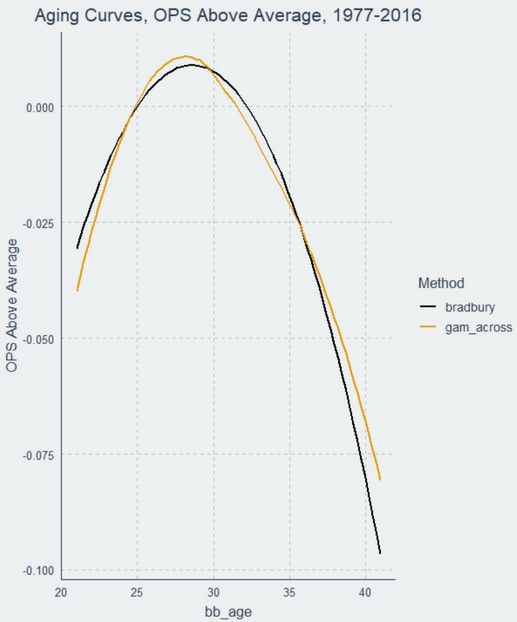
The two curves are similar, and in fact their test scores (which you can discover in our R code) are almost identical. This means that the Bradbury curve works just fine overall, and like the GAM Across method, appears to provide just as good if not better explanations for aging on average than either delta method.
However, because both slopes of the curve must be identical, the Bradbury model ends up pushing the “peak” of its parabola over to age 29 to enforce that symmetry. The effect of this is not substantial in the aggregate, but it does end up giving what I believe to be a wrong answer in this one respect. This is one reason why GAMs have largely supplanted quadratic regression models in statistical analysis: GAMs do not require symmetric curves.
Now that we have tackled Team Bradbury, let’s focus on Team Delta. Over our 1977 through 2016 time frame, both delta methods estimate that players reach their peak performance at age 26.[5] Why do I disagree with this? Because this probably reflects when the average rate of major league performance peaks, not when the average major-league player peaks.
To understand why, take all major-league position players from 1977 through 2016 and determine for each one of them the age for their highest OPS above average. It turns out that baseball careers, on average, hit that highest OPS at 27. We can do this using the median also, which arguably represents the “typical” instead of just the average player. The baseball age when the median player hits their highest OPS above average? 27.
However, the delta method reports above that the peak batting age for hitters in this cohort is 26, not 27. This suggests that the delta method might have a unique bias of its own. Can you guess what it is? Here is a hint:
The bias here is not with survivors, but with new arrivals. The earlier you start your MLB career, the better you are on average. Because these players are overrepresented in the earlier age groups, the average overall MLB performance can peak earlier, while at the same time that overall average performance, driven primarily by above-average players, is not actually representative of average MLB players, who tend to arrive later.
As noted above, the Bradbury model compensates for this by controlling for career-average performance, but is hampered by an overly-restrictive quadratic model. The GAM Across model also controls for career-average performance. However, because of its additional flexibility, the GAM Across model seems to reach the best answer.
The difference between these peak ages is somewhat academic: nobody is going to cut an average player just because he turned 29 (particularly since the best players tend to peak later, despite arriving in MLB earlier). Average MLB players are incredibly valuable, and find their way onto a roster almost regardless of their age.
Nonetheless, this underscores that one of the trickiest issues in evaluating any model is figuring out exactly what question the model is specified to answer. Frustratingly often, it is not the question we intended to ask.
Conclusion
We conclude that semiparametric regression, also known as a generalized additive model or GAM, may perform just as well, and possibly better, than either the traditional “delta” method or Lichtman’s proposed corrections to it. Furthermore, GAMs provide additional advantages over previously-standard parametric methods such as quadratic linear regression. Semiparametric regression does not require reorganization or disposal of data, and its results are virtually instantaneous for models like these on modern hardware. To achieve sensible results, the analyst must still control for the career-average performance of every batter.
The GAM we proposed here is a floor, not a ceiling. We see no reason why the use of semiparametric regression should not be standard practice in aging research, but we absolutely can and do encourage readers to strive for better than the model we featured here. More sophisticated GAMs have already been proposed, and GAMs can be used with seasonal pairs as well. Further progress may require that we rethink some of the fundamental assumptions that guide current aging curves. We expect to be discussing that issue in the near future.
We have made R code in our Github repository available that allows you to reproduce the findings of this article and to alter its assumptions. Among other things, you can change the seniority and experience level of players considered.
[1] Not to be confused with the delta method of calculating standard errors.
[2] This topic could take up a separate article.
Briefly, in our last article, we used simulation to investigate the effect of possible survival bias on baseball aging research. We found that, with respect to our ability to recover aging effects, survival bias either doesn’t materially exist at all or if it does exist, that it causes the pool of survivors to understate, not overstate aging effects. What Lichtman describes does not fit into either of these categories.
Moreover, the asserted premise of this correction is that major league teams are cutting players who were merely unlucky in their most recent season even though their projections suggest they would perform better next year. It would be very odd for a major-league club to behave this way. If anything, many clubs would target these players as bargain signings. If one club cut such a player, others presumably would seek to sign him.
To the extent some version of this problem actually exists, it may be a problem unique to the delta method. As far as I can tell, this correction ultimately is a shrinkage function that uses projections for departed players as the mechanism of choice. The statistical justification for the correction is unclear, but I am more puzzled by it than critical of it. I would welcome a better or alternative explanation for its usage.
[3] We provide a link to code that does this automatically at the end of this article.
[4] During our tests we marginalized out player career means from our predictions, so only age was being used to forecast performance.
[5] The typical peak age can move around if you include other seasons, as was the case for earlier analyses, and different skills can have different peak ages. However, the relative quickness or lateness of the suggested peak between the methods discussed should be fairly consistent.
Thank you for reading
This is a free article. If you enjoyed it, consider subscribing to Baseball Prospectus. Subscriptions support ongoing public baseball research and analysis in an increasingly proprietary environment.
Subscribe now
Thanks for reading!
I've had a nit to pick with these types of analysis for a long time: anything using OPS. I love OPS, am fine with using OPS for regular type of discussions (i.e. fan discussions), but with broad based long history data sets like this, and the ability to use the computer to do computations, I'm surprised I don't see more analysts using OBPxSLG (Bill James original metric) as the valuation metric, instead of OPS, especially with hitters going more towards 3 True Outcomes type of hitting. And it could just be indexed vs. the overall majors OBPxSLG, so one doesn't have to adjust their thinking seeing .160 as a good metric.
The thing is, the more "balanced" hitters (whose OBP and SLG are relatively close to each other) is getting undervalued relative to the 3 True Outcome types. Here is an example of what could happen: two hitters, both .800 OPS, but one is .400/.400 and the other is .300/.500. By OPS, obviously, they are the same. But using OBPxSLG, one gets .160 for the former, .150 for the latter, so the first hitter is 6.67% better but using OPS makes him equal to the other hitter. It may not seem like much but if the latter is truly .800 OPS, a 6.67% better hitter is a .853 OPS hitter. That's going from about average corner MLB OF, to a top 20-25 OF.
Or, say, the same first hitter, .400/.400, and a second hitter, .313/.512. The second hitter would be .825 OPS vs. .800 OPS, looking the better hitter, by a good bit, but both are .160 using OBPxSLG, meaning they should be equal, roughly.
If the mix of hitters over the years are roughly the same mix of hitters, in terms of their SLG-OBP difference, then it would not change the results much, it seems to me. But if hitters have been changing to be 3 True Outcome hitters, as I believe, then that would change the analytical results, I believe.
In general, these curves need to be applied to specific components like strikeouts, walks, home runs, and the like, and from there we can give additional insight on questions like this. But first . . . we need an understandable example to see it in action.
For now, with this very basic aging curve, the answer would be to assume that your player, even if he improved from 27 to 30, would still on average be expected to trend downward at the rate the GAM Across curve indicates for all players at 31 and above.