
Aging effects can be important when evaluating player performance. Aging patterns inform us when players typically start to be effective, produce their peak contributions, and offer diminishing returns. These effects are commonly summarized by a so-called “aging curve,” which estimates the average growth and decline of players over time. Different skills can have different aging curves, even within the same sport.
One challenge in developing an aging curve is that the players we see on the field rarely represent the entire population of possible players. Sometimes, we have survivor bias, when there are additional players who might be playing, but who either choose not to play or are not chosen to play.
This study uses simulation to evaluate the potential for survivor bias with batter on-base-plus-slugging (OPS) in Major League Baseball. Simulating across several scenarios, and focusing on players 31 to 35 years of age, we find that the existence of survivor bias depends upon the shape of the talent distribution of the players who drop out. If the dropouts effectively form their own bell curve distribution of talent, we have a mixture distribution composed of two pools of players. If the dropouts instead represent the bottom of one overall skill group, we have a truncated distribution that covers both survivors and dropouts.
In the mixture distribution scenario, there may be no meaningful survivor bias at all for aging estimates, even when we exclusively measure surviving players. When the distribution is truncated, we confirm survivor bias that underestimates aging effects. However, we show that this bias can be controlled by adjustment, allowing us once again to accurately estimate OPS aging effects solely from surviving players in the Major Leagues. We conclude with discussion and additional recommendations.
Previous Treatments
Survivor bias is a topic that many people warn about but few attempt to solve. This may be because analysts think it is not capable of being solved. As such, our literature review will be quite short.
One person who has thought about survivor bias extensively is Mitchel Lichtman, while employing what he calls the “delta method” of aging. This delta method uses historical data, tabulating the average change across baseball for all batters with consecutive seasons (i.e., “seasonal pairs”). By considering only batters with paired seasons, the delta method imposes selection bias. Lichtman contends that this selection bias is also survivor bias, and further contends that it causes the delta method to overestimate aging effects.
To address this, Lichtman suggested imputing the hypothetical performance of player dropouts through projection, based on their past performances. In a later article, Lichtman proposed a variant of this approach that makes a more dramatic correction.
CJ Turtoro, in the context of professional hockey, found that imputing performances for players who dropped out did not improve the accuracy of performance prediction for those who remained.
This article will focus on theoretical limits rather than particular empirical corrections, and on structural effects of survivorship that transcend particular methods of measuring aging effects. The larger point is that disappointingly few efforts have been made to address the potential for survivor bias, at least in baseball analysis.
Our Approach
We use simulation to evaluate a range of situations where survivor bias could be problematic in measuring aging effects. Specifically, we analyze simulated batter OPS from ages 31 to 35; those ages cover a time period of consistent decline in performance and many player dropouts.[1]
Simulation is necessary because we cannot observe players who drop out in the ordinary course: you cannot observe a player who does not play.[2] Thus, in order to “observe” such performances, we need to make them up. This works because we are not trying to forecast particular performances; rather we are trying to figure out whether the range of likely performances would actually create any problems. We accomplish this by simulating different performance levels and gaps between survivors and dropouts, and seeing which combinations result in survivor bias and which ones do not.
First, we state our primary assumptions.
Assumption 1: Not all capable players are observed.
In addition to being the entire premise for this article, this assumption seems reasonable: some players get hurt, others get cut for a newer model, others retire, others go overseas, and still others just aren’t good enough to play at a big-league level anymore.
Assumption 2: Observed players are expected to be better than those who drop out.
This assumption also seems reasonable: Clubs are trying to win, so they keep players they think will help them win and cut players they think will not. Of course, teams sometimes make mistakes, or choose players based on criteria other than expected batting performance (e.g., defensive needs). So, the cut players are expected to perform worse than surviving players on average, but there could be overlap in expected OPS between the two groups.[3]
Assumption 3: Even players of different abilities share an average overall aging pattern.
This might seem like a bold assumption, but it may not be. The very notion of an overall aging curve assumes this commonality: we are just being explicit about it. This does not preclude the existence of “subgroups” that age differently, but even a group of subsets must have an overall average trend.
What should we assume that overall aging effect might be? You could assume that a surviving big league player loses on average about five points of OPS per year from age 31 to age 35. (This is Ray Fair’s estimate; it might be a bit on the low side).
We have already assumed that we have a pool of dropouts and that these players have a lower expected OPS on average than our survivors. It’s possible our dropouts have a faster rate of aging as well. We don’t know this, but it is possible. Dropouts also may age slower if they have less of a decline to make in the first place. We don’t know that either.
But we do know that a “true” overall aging rate for all players would necessarily be a blend of the survivors and the dropouts, even if their aging rates are different. We also know that from age 31 to 35, the pool of big league players shrinks by about 20 percent each year. So the overall pool is going to be weighted toward the survivors. Thus, even if dropouts end up with a very different aging rate, their ability to affect the overall curve on average should be somewhat limited.
We can, and do, hedge our bets by testing a range of average aging effects that, overall, would govern both survivors and dropouts.
Our Simulation
Pursuant to these assumptions, our simulation will be based on two hypothetical sets of batters: (1) a group of survivors selected to play in a given season, and (2) a group of dropouts not selected to play. The difference between these two groups will be in their expected performance: Players who are selected are believed on average to be better hitters. We don’t care whether the players ultimately play or not, because again, we are basing this on expected performance only.
Simulation allows us to address the core question: Does considering only surviving players bias our aging analysis? We answer this by specifying a possible aging effect up front, and then seeing how well we recover that effect if we work backwards, first with the non-surviving players included, and then excluded like they normally are in the real world. Any differences we recover from the original values indicate bias. More importantly, we assess whether any bias we do see is large enough to make any difference.
To do this, we created a dataset of expected major league performances with the following characteristics:
- Survivors: We simulated 2,000 raw performances by random draw from a normal distribution with a mean OPS of .740 and a standard deviation of .08. This approximated the major league average and standard deviation for survivors in our designated age group of 31 to 35.[4] We use OPS because, although it is not best-in-class among batter statistics, it still does a good job estimating productivity and is well-understood by most readers.
- Dropouts: We then simulated 500 additional raw performances drawn randomly from the same distribution as the survivors, but which were penalized by a constant we subtracted from this initial OPS. We’ll call this the dropout delta. This effectively shifts the midpoint of their distribution downward relative to the survivors. In different simulations, we varied this delta from 40 points to 300 points to see if the difference mattered.
- Each raw performance was then randomly assigned an age between 31 and 35, and the final expected performances reflected the penalty that corresponded to the assigned age. So, a player’s Age-31 performance reflects the baseline aging penalty, Age-32 reflected twice that aging penalty, and so on.
The 80-20 ratio for our survivors versus dropouts is intended to mimic a 20 percent dropout rate for this age group.
We test the following deltas between average expected performance for survivors and dropouts: 40 points, 100 points, 200 points, and 300 points. Forty points is the approximate delta between the career average OPS of players who tend to stay and those who tend to drop out during this time period. It is a very conservative number to use, which is why we test higher deltas as well.
With respect to aging, we test the effect of the overall group losing an average of five points of OPS per year, 10 points per year, and even 20 points per year.
To test for bias in age measurement, we used linear regression models.[5] To remain method-agnostic, we will keep player data in its native format and not rely upon “seasonal pairs.” For each scenario, we regressed expected OPS on age for all performances (survivors and dropouts) and then ran a second model with the same specifications but which contains survivors only. Normally-distributed errors were assumed for both models.
To minimize the risk that any one simulation was unrepresentative, we resampled each scenario 50,000 times and averaged the results over all of them. Monte Carlo standard error for all estimates was .00001 or less.
Scoring
Our scoring methods are bias and mean squared error (MSE).
To determine bias, we test our ability to recover the aging penalties we specify from both our theoretical survivors and our dropouts. If we have avoided survivor bias, we should recover the same average aging effect from the survivors as we do from the combination of the survivors and the dropouts.
Arguably, the more important measurement is the MSE. To concern us, the biases must be substantial enough to overcome the natural variance in the system. In other words, if the bias at issue is so small that it gets swamped by variance, then very small biases may not affect player projections, even if they technically do exist. The MSE addresses this question for us.
Let’s begin with our conservative estimate of an aging effect: Five points lost per year for all players, surviving or not.
Scenario One: .005 aging penalty (5 OPS points per year on average across all batters)
|
OPS Pool Gap |
All Performances |
Survivors Only |
||
|
Bias |
MSE |
Bias |
MSE |
|
|
40 points |
-.00001 |
0 |
-.00001 |
0 |
|
100 points |
-.00001 |
0 |
-.00001 |
0 |
|
200 points |
-.00001 |
0 |
-.00001 |
0 |
|
300 points |
-.00001 |
0 |
-.00001 |
0 |
The first column is our bias measurement, defined as distance away from the “true aging” penalty we specified above (-.005 or 5 points of lost OPS per year). Again, our goal is to recover that value when we work backwards through our model. If the recovered bias is over 0, that means it reflects a positive bias and is not penalizing players in that group enough; if it is less than 0, it is a negative bias and is penalizing players in that group too much.
Here, both the “all players” group and the survivors-only group show the same amount of trace negative bias. But even with an average performance gap of 300 points of OPS (which is unrealistically large), the results do not become materially biased. We know this because the MSE for all models is zero, meaning that everyday variance swamps this nominal bias, and the bias simply does not matter.
This suggests that survivor bias could be a non-issue for OPS, provided the aging penalty is small on average. What if the aging penalty is larger? Let’s double it.
Scenario Two: .01 aging penalty (10 OPS points per year on average across all batters)
|
OPS Pool Gap |
All Performances |
Survivors Only |
||
|
Bias |
MSE |
Bias |
MSE |
|
|
40 points |
-.00001 |
0 |
-.00001 |
0 |
|
100 points |
-.00001 |
0 |
-.00001 |
0 |
|
200 points |
-.00001 |
0 |
-.00001 |
0 |
|
300 points |
-.00001 |
0 |
-.00001 |
0 |
The numbers are . . . exactly the same. Doubling our annual overall aging effect did not have any effect whatsoever. So let’s double it again.
Scenario Three: .02 aging penalty (20 OPS points per year on average across all batters)
|
OPS Pool Gap |
All Performances |
Survivors Only |
||
|
Bias |
MSE |
Bias |
MSE |
|
|
40 points |
-.00001 |
0 |
-.00001 |
0 |
|
100 points |
-.00001 |
0 |
-.00001 |
0 |
|
200 points |
-.00001 |
0 |
-.00001 |
0 |
|
300 points |
-.00001 |
0 |
-.00001 |
0 |
More of the same. Under the conditions of our simulation, the inherent variance in the system swamps any potential bias, even at an aging effect of 20 points per year, which would be very large.
Does this mean, at least with batter OPS in baseball, that survivor bias is a complete non-issue? Possibly.
Except there is one catch. There always seems to be a catch.
The Truncation Problem
You may recall that earlier we identified two patterns that can describe pools of dropouts versus survivors. The first is what we have been analyzing so far. I described it above as a mixture distribution: this name comes from the fact that it is composed of two separate distributions, one for survivors and one for dropouts, which tend to overlap (the dropout delta dictating how much overlap there is).
This is easier to understand through illustration. Here is one simulation of how a mixture distribution would distribute survivors versus dropouts from ages 31 through 35, with a dropout delta of 200 points of OPS and an average aging penalty of 10 points per year:
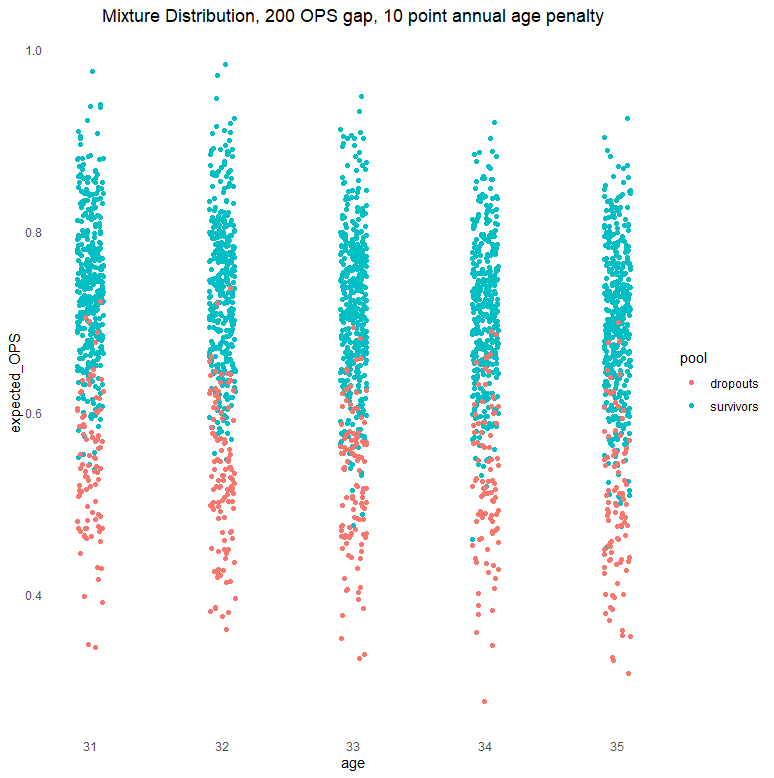
Clearly, the dropouts are expected to be less capable on average than the survivors. There is also some overlap. Regardless, both groups are distributed over their respective spectrums, and that seems to be what matters. As we showed above, even though the average expected performances between the two groups are quite different, we can recover the true aging penalty even if we look only at survivors.[6] This is the best possible outcome. I suspect many readers are shocked it is even possible.
But survivors and dropouts can also arrange themselves in another way. Picture a league in which a certain type of player is defined by one primary skill, the player is easily replaced, it is easy to measure whether the player is performing well, there is widespread consensus on those measurements, there are no contractual complications, and players are bounced out of the league the moment they are no longer expected to perform well. Then you might end up expected performances that are distributed like this:
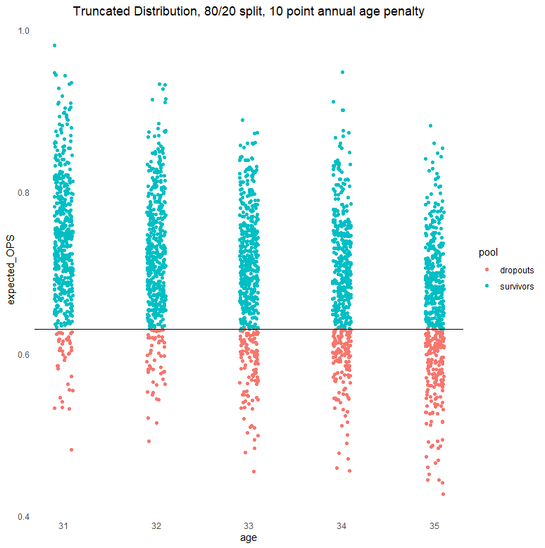
This is known as a truncated distribution: We still have an 80/20 split, but it is enforced at a fixed performance level, as indicated by the horizontal line. Everyone above the 20th percentile line stays and everybody below the line goes. The nice distributions we had before, including some overlap between pools, are replaced by concentrations exclusively in different parts of one overall distribution, both now with an irregular shape. If we try to run the same models as before, which assumed normally distributed errors, and run them only on survivors, we end up with significant survivor bias:
Scenario Four: Truncation (80/20 split, various aging factors, standard models)
|
Aging Penalty |
All Performances |
Survivors Only |
||
|
Bias |
MSE |
Bias |
MSE |
|
|
-.005 |
0 |
0 |
+.00208 |
+.00001 |
|
-.01 |
0 |
0 |
+.00411 |
+.00002 |
|
-.02 |
0 |
0 |
+.00792 |
+.00006 |
The “all players” group, which we can’t fully observe in the real world, has no bias. The survivors-only group, which we do observe, now has significant bias.[7] Interestingly, the bias causes us to underestimate, not overestimate, aging effects. Specifically, the aging penalty we recover is positively biased, understating the aging penalty by 2 points of OPS for each year of age at the -.005 penalty level, 4 points for each year of age at the -.01 level, and 8 points for each year of age at the -.02 level. On average, the 80/20 truncation causes us to underestimate aging effects by about 40 percent. Informal testing of other truncation levels suggests that the amount of bias is a function of the amount of truncation, which makes sense.
Admittedly, the MSE is much smaller so perhaps one could argue this bias doesn’t matter. Fortunately, we don’t have to entertain that argument, because there is a solution for this truncated distribution too.
As it turns out, the ingredients that make a truncation so challenging to fit with ordinary tools also give us the clues to solving it in another way. We know that on average 80 percent of the players in this age range stay and 20 percent of them drop out. That means we also know that the distribution of survivors, while biased, is also only the top 80 percent of what it ought to be and what we expect we would see if the dropouts had been allowed to perform. And because we assume that errors from the full distribution would have a quasi-normal character, we can turn to the truncated normal distribution to fill in the gaps for us. We specify that the truncation begins at the 20th percentile.
When we re-run our models now, assuming this truncated error distribution, look what happens:
Scenario Five: Truncation (80/20 split, various aging factors, with truncation correction)
|
Aging Penalty |
All Performances |
Survivors Only |
||
|
Bias |
MSE |
Bias |
MSE |
|
|
-.005 |
0 |
0 |
0 |
0 |
|
-.01 |
0 |
0 |
-.00002 |
0 |
|
-.02 |
0 |
0 |
-.00004 |
0 |
The problem is addressed. The bias is once again minimal, and as indicated by the MSE, it is ignorable. Provided we have a sense of the overall distribution of survivors and dropouts taken together, the survivors alone can tell us what we want to know about player aging.
While it is nice to know we can solve the problem either way, it is more important to know which scenario better describes your particular sport and statistic. If truncation is at work, it can be noisy, because not every player who performs well enough to survive chooses to stick around, and teams don’t always choose players for entirely hitting-based reasons. The noisier the truncation is, the more it may gravitate toward the mixture distribution on which we have focused much of this article. However, a general truncation effect could still be in place, at least for certain statistics / skills, and a mixture distribution can certainly be noisy in its own right. Of course, if what you have is fundamentally a mixture distribution in the first place, this all becomes much easier.
Furthermore, different statistics may have different distributions for dropouts, and those distributions could change over time depending on the nature of the statistic / skill and the changing values teams place on it. It is imperative that the analyst check these trends and distributions, rather than merely assume they operate in a desirable way.
Finally, it is possible that imputation of dropped-out players, carefully done, could recreate the true distribution in a way that obviates the need for a truncation correction. But this should not be taken for granted. It is possible that imputation could aggravate existing problems or create new ones, particularly if the imputation inputs are themselves confounded by aging.
Conclusions
We have shown, perhaps surprisingly, that fears of survival bias in measurements of baseball aging effects may be unfounded, at least under conditions analogous to those studied here. Under those same conditions, we have further shown that when survivor bias does arise, it can also be overcome, permitting aging effects to be estimated from surviving players alone.
We think the findings of this study are exciting. But they should be applied with care. Before scrutinizing trends in player ability, the analyst should carefully think through the problem of interest, using her expert knowledge of the subject area, to determine which distribution (or further mixtures of distributions) best characterizes the relationships between survivors and dropouts in the sport and statistics at hand. The analyst should then use simulation to confirm that survivor bias can be appropriately neutralized or avoided under those circumstances. In other words, do not blindly apply a “correction” under the assumption that survival bias exists. You may be correcting for a problem that does not exist, or correcting in the wrong direction or in the wrong amount if it does exist. This makes your estimates worse, not better.
The findings of this article could also be seen as consistent with causal inference. The mechanism envisions age having an effect on expected performance which in turn results in a selection mechanism that potentially causes survivor bias. External information, such as knowledge or expectations for the overall population, can sometimes help, conditional on the reasonableness of such information. As is often the case, expert knowledge and judgment plays a crucial role in defining the bounds of the problem and potential solutions for it.
We view this study as the beginning, rather than the end, of our efforts to better understand survivor bias in baseball. There are other aging phases of interest besides ages 31 through 35. The effect of playing time may allow for more nuanced comparisons. Dropout distributions would benefit from further study, including analysis of the sensitivity of their assumptions, the consequences of breakdowns in those assumptions, and the spectrum that exists between different distributions and the effects of those differences.
Although we used OPS as our example statistic, we could have used pretty much anything. Thus, while our findings do not automatically generalize to other sports or even other baseball skills, we suspect they will replicate in other applications. We hope that these replication efforts occur, and that readers will keep us posted on them, because there is much we can learn from other sports and applications.
For that reason we have provided, at our Github repository, the R code that allows you to reproduce our findings and adapt them to your area of interest.
Special thanks to Rob Arthur, Greg Matthews, CJ Turtoro, and the BP Stats Team for helpful insight and suggestions, and to many other reviewers, internal and external, for their comments.
[1] Other age ranges matter too, but we will build intuition with something more limited to start.
[2] We will put to one side the possibility of translating statistics for players who proceed to play in other leagues, domestically or overseas. This is another source of potential information, albeit one that can be complicated by additional sources of bias.
[3] The existence (or non-existence) of this overlap, as we will see, can be important.
[4] The particular OPS doesn’t really matter, but you do have to pick something, and it might as well be something in the ballpark of the group being studied.
[5] For many scenarios, you get a similar answer by subtracting the average of the samples for survivors only from the combined average of the samples combining survivors and dropouts. However, that approach does not work for truncation, and regression does, so we use regression throughout.
[6] In the missing data literature, this means that these dropouts are “Missing at Random” (MAR): their missingness is conditional on other observed variables, but their missingness mechanism is ignorable.
[7] Without correction, dropout performances here would be considered “Missing Not at Random” (MNAR) in the language of the missing data literature, and we would be in trouble.
Thank you for reading
This is a free article. If you enjoyed it, consider subscribing to Baseball Prospectus. Subscriptions support ongoing public baseball research and analysis in an increasingly proprietary environment.
Subscribe now