Abstract
This post confronts a familiar problem: the need for speedier estimation of Bayesian inference. Markov Chain Monte Carlo (MCMC) provides superior accuracy with reliable uncertainty estimates, but the process can be too time-consuming for some applications. Oft-recommended alternatives can be unacceptably inaccurate (posterior simulation) or fail to converge (variational inference). To help fill this gap, I propose a Bayesian block bootstrap aggregator to estimate uncertainty intervals around (transformed) group-level parameters, as computed by the (g)lmer function of the lme4 package in the R programming environment.
The procedure estimates the spread of the posterior for group members by sampling with replacement from a Dirichlet distribution in blocks of taken pitches from entire plate appearances. The model is re-run on each set of resampled data, and the modeled (and transformed) intercepts are then aggregated to create an approximate posterior for all modeled groups. In a fraction of the time required for full MCMC, this Bayesian ‘bagging’ procedure can reasonably estimate the uncertainty around the most likely contributions of catchers in framing borderline baseball pitches. The similarity of this process to frequentist bootstrapping should make it approachable for practitioners unfamiliar with Bayesian estimation.
Late last year, the baseball analysis community got its knickers in a twist over the appropriateness of using wins above replacement player (WARP or WAR) as a proper means of evaluating the most valuable players in baseball. Although many focused on whether player run value was better estimated with respect to actual team wins versus league average wins, our takeaway was different: the problem, we concluded, was not how an analyst chose to value to win contributions, but rather that readers currently have no objective basis by which to mathematically distinguish players from one another.
To use Bill James’ example, by Baseball Reference’s system, Jose Altuve was worth 8.3 WAR during the 2017 season, whereas Aaron Judge was worth 8.1 WAR. But what does that mean? Are those two numbers really different? If the season were to be replayed 10 times, would we expect their alternative results to be the same? Would Altuve and Judge exchange places? If so, how often? Could they tie?
This, for us, is the real problem. The issue is sometimes framed as a debate over precision, but the real issue is that analytic websites generate slews of numbers without telling you, the reader (and often enough, even the authors) whether the differences in numbers assigned to players are meaningful. The gulf between best and worst may be fairly evident, but most players are not so obviously different over the course of a season.
The elephant in the room is uncertainty, which is odd given that accounting for uncertainty is what the field of statistics is supposed to be all about. Yet, sports websites routinely ignore uncertainty, presenting calculations without any estimates as to how wrong they could be. Much like election pundits, sports analysts instead advise that “one should never rely on one statistic alone” or by declaring the difference between two players “probably too close to call,” but never with any real accountability for how uncertain their (assumed) estimates are. (This list of analysts includes us.)
There can be many reasons why websites shy away from uncertainty estimation. One is the belief that readers really don’t care about uncertainty. Another is resource-based: estimating uncertainty requires additional (daily) resources and demands more columns on already-crowded tables.
But I think the primary reason is that estimating uncertainty is hard. Moreover, even when a method is selected, resources remain an issue: even in the cloud age, most websites have only so many cores available for simultaneous computation, and only so much time to push the daily refresh enthusiasts expect to see each morning.
I think we have a solution to at least some of these problems. What follows is our proposed approach, which we will deploy first for our catcher framing statistics. We chose catcher framing as a test bed because it is an area of particular emphasis (and expertise) for Baseball Prospectus, and one that seems particularly well-suited to uncertainty calculation. Catcher framing has a high profile in baseball, as the difference between a good and poor framing catcher — even today — can range up to 50 or 60 runs. On average, that amounts to several potential wins over the course of a season. For teams on the cusp of postseason contention, the marginal value of catcher framing can therefore be substantial, and must be weighed against other catcher skills to determine the best fit for team resources. For example, a catcher with a great bat may be a better bet than a catcher with positive framing skills, but great uncertainty around those skills. Mere point estimates, which is all most websites have provided to date, cannot help with that decision.
Below, we provide our material code in R, along with our reasons for using it. Our hope is that others will evaluate, criticize, and suggest improvements to this approach, both from inside and outside the sports analysis community. Good resources for estimating uncertainty are hard to find, and worthwhile debates over methods are even more scarce. Whether employed in fantasy drafts or real-world decisions, we think that being more honest about uncertainty will make our readers better consumers of sports and other information.
I. Foundations
A. A Multilevel Framing Model
Our baseline for this effort will be our catcher framing model, which we published just over 2 years ago. Before we get to quantifying the uncertainty around that model, we’ll briefly discuss the model to which we are applying it.
Catcher framing was one of the first subjects to which BP publicly deployed multilevel modeling, an approach that has become the de facto standard for sophisticated regression analysis in many academic fields. Also described as “mixed models,” “random effects” models, “hierarchical” models, or “mixed effects” models, multilevel models use the power of parameter groups to achieve more accurate results. In an era where deep learning and boosted trees capture most of the headlines, multilevel models demonstrate that parameters, and especially the uncertainty around those parameters, still play an important role in statistical learning.
Briefly, multilevel modeling applies a ridge penalty to value different members of a group relative to each other, thereby accounting both for each member’s results and the number of opportunities each group member had. This second “level” of analysis operates in addition to the usual inclusion of more universal covariates (a/k/a “fixed effects”) that also correspond to the outcome of interest. In a catcher framing model, we look not only at whether a taken pitch was a called strike, but also the groups that we know can affect that pitch: the catchers, the pitchers, the umpires, and the batters. (We track the performances of all four groups, although catchers receive by far the most attention from the baseball analytic community). The model tracks not only how each catcher or pitcher performs, but also how they perform relative to other catchers and pitchers, over a scaled unit-normal prior distribution. Players with smaller samples are shrunk substantially toward the overall mean, whereas players with larger samples and/or more extreme results are permitted to stand out and populate the tails of the distribution for each group, albeit still with some shrinkage. The overall result is predictions that are more accurate, and inferences that attribute credit more conservatively to individual players.
A catcher framing model therefore has three general types of predictors: (1) the expected called strike probability of the taken pitch, based on the pitch’s projected location [this is separately and previously calculated]; (2) the groups of relevant participants to that taken pitch; and (3) factors that are viewed as applying similarly to all participants. The first aspect controls for the likelihood of the pitch being called a strike regardless of participant; the second allows the various participant groups to be credited (or debited) by their most likely contributions to the result; and the third recognizes that strike calls to some extent reflect both home field advantage and the closeness of the game, our “population” covariates of choice.
Catcher framing is an excellent demonstration of why multilevel models matter. Over the course of the 2017 season, major league baseball featured 110 catchers, 941 batters, 748 pitchers, and 94 umpires. Good luck fitting that with your generalized linear model. Moreover, it is extremely unlikely that there are 110 different levels of performance among catchers, much less 748 different ways for pitchers to throw strikes on the corners. A multilevel model recognizes this, and uses shrinkage not only to compress the differences between players into a more reasonable range, but also to borrow strength from the other groups being subjected to similar processes. More reasonable estimates of catchers in turn allow more reasonable estimates of pitchers, which allow more reasonable estimates of umpire effects, and so on.
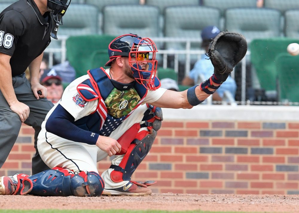
In R, using the conventional lme4 notation, a standard catcher framing model could be specified like this:
The variable cs is our output variable, whether a strike was called; half_sc and run_diff_sc reflect the home field advantage and score differential respectively (scaled to the unit normal); the four participant groups a/k/a “random effects” are specified in the (1|x) format; the family is specified as the probit link, which is consistently more accurate than the canonical logit for ball / strike applications. (Comparing a probit posterior to a logit posterior with LOO, the probit model was preferred in our 2017 model with an elpd_diff of 1080 and a standard error of just 14. If you compare maximum likelihood models, similar findings of superiority result from likelihood ratio tests, accuracy comparisons, and information criteria. Don’t just default to the logit when using binomial models, folks: it’s lazy. Check all of the available link options.).
The R package lme4, which is how we calculate our current framing model, uses penalized likelihood and uniform priors to speedily process even large data sets with multiple large groups. (With 300,000+ observations, this model takes only about 10 minutes to analyze a season on a core-i7 processor). Lme4 is used by frequentists and Bayesians alike who seek quick answers to standard multilevel problems. However, lme4 does not automatically provide uncertainty estimates around its varying intercepts, and the supplemental tools it does provide – like bootMer – are very limited in what they can do.
We can say a lot more about catcher framing, but framing is our departure point, not our overall point, so let’s proceed.
B. The Need for Bayesian Approach to Uncertainty
The most common means of reporting uncertainty is to provide an upper and lower bound around the projected (mid)point estimate for a statistic. When the uncertainty around a statistic is normally distributed, a standard deviation (a/k/a “margin of error”) is usually sufficient, as any interval of the reader’s choice can be estimated from the standard deviation.
Our most important rule for these uncertainty estimates is that they be useful — not just in general, but useful for the applications to which readers will try to use them. In that respect, there is little doubt what a reader expects when she sees a statistical estimate (typically a mean or median) surrounded by an uncertainty interval: that the “true” value of the estimate lies somewhere in between, and most likely at the chosen midpoint.
Unfortunately, that is not what the intervals reported by most statistical analyses actually mean. Reflecting the historical prevalence of frequentist thinking, the vast majority of reported uncertainty estimates are so-called “confidence intervals,” which cannot be interpreted in that common-sense way. In fact, one of the standing jokes in statistics is that many people struggle to remember how confidence intervals should be interpreted. This includes some of the brightest people who teach statistics; published authors sometimes get it wrong too, as do researchers and of course students.
According to Wikipedia, “[t]he confidence level is the frequency (i.e., the proportion) of possible confidence intervals that contain the true value of their corresponding parameter,” which “does not necessarily include the true value of the parameter.” The definition makes “sense” in that it fairly describes an important limitation of so-called frequentist inference, which is that one cannot ever know the “true” value of any parameter. But for our purposes, we believe that traditional confidence intervals are essentially worthless, if not actively misleading: a reasonable reader will naturally interpret them in the opposite manner in which they are intended, whatever your contrary footnote may assert. To be sure, confidence intervals can be useful in general, are well established in the statistical literature, and have been rigorously implemented in important studies, such as OpenWAR, by excellent statisticians analyzing baseball events. But for our purposes, I believe that giving readers “confidence intervals” around our statistics would be a serious mistake that could undermine, rather than encourage reader reliance.
There is an alternative: the so-called “credible interval” of Bayesian statistics. Under Bayesian philosophy, parameters are estimated through conditional probability, rather than a likelihood function alone. This means that a credible interval can be interpreted in exactly the way the reader would expect: A median estimate of 10 runs saved, in the midst of a credible interval of 6 to 12 runs saved, means that, conditional on the data and model, we estimate that the true value of the runs saved by that player is between 6 and 12 runs. No gobbledygook, and no qualifications: what you see is what you get. That doesn’t mean Bayesian models cannot be wrong, but it does mean that our likely mistakes are confined to the range of the interval. The term “credible interval” is traditional, but we agree that the term “uncertainty interval” is more clear (and also less self-congratulatory). Going forward, we will refer to our intervals as “uncertainty intervals.”
However, this requires that we adhere to Bayesian methods in providing our framing analysis: if we want to have true uncertainty intervals, we must follow Bayesian rules and derive our estimates using conditional probability. These requirements are somewhat more rigorous, but the good news is that this is our problem, not yours. If we do our part, the reader is free to rely, in a common-sense way, upon the standard deviations (or other intervals) we supply around our statistics.
Let’s talk now about how we propose to do that.
II. Generating Uncertainty Intervals around Framing Value
Bayesian methods require two primary things: a prior distribution on the parameters of interest, and a posterior probability distribution fit to those same parameters.
The most established, straightforward, and (typically) accurate way to do that is with Markov Chain Monte Carlo (MCMC).
A. Uncertainty Estimates with MCMC
Stan is a probabilistic programming language designed to, among other things, harness the power of Hamiltonian Monte Carlo to provide efficient sampling of target distributions. Headlined by the No-U-Turn-Sampler (“NUTS”), Stan offers fully-Bayesian estimates. Because Bayesian analysis works through distributions rather than point estimates, uncertainty intervals of any size can be directly quantified from the model posterior.
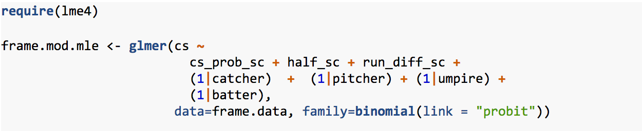
Stan itself is programmed in C++, and thus is accessible from many programming languages, but users of the R programming environment are blessed with an array of front-end tools that substantially simplify the task of harnessing Stan’s power. In particular, the Stan team has created rstanarm, a front-end that allows users to generate Stan models using R-standard modeling formats, including that of lme4. Thus, in rstanarm format, the same framing model from above can be re-specified in this way, to run in Stan:
After loading the two required packages, the first three lines of the model are the same as before, with the addition of the prefix stan_ before the glmer function, as is typical for rstanarm. After that, we specify the desired number of chains and cores (4 for both), which is useful on a multi-core machine to distribute the load and help ensure convergence.
Bayesian inference requires the specification of prior distributions, but this has become much more straightforward in recent years as priors are increasingly used for regularization rather than for personal declarations of belief. Stan also makes prior specification easier because it does not require priors to be “conjugate,” a typical requirement of previous methods that substantially complicated the process of compiling a Bayesian model, and sometimes provided wonky results. As a practical matter, the number of observations in a full-season framing model is so large (over 300k) that the priors really don’t matter. But, it is good practice to specify priors anyway to help direct the Markov Chains to the right place. For our purposes, we’ve largely stuck with the default values, but specified them anyway (again, good practice). We placed a wide normal prior on the intercept, a mildly-regularizing prior on all non-modeled parameters (a/k/a “fixed effects”); an exponential prior on the standard deviation (prior_aux), and a lightly-regularizing prior on the correlation matrix of our group coefficients; again, these priors largely wash out with the data. The adapt_delta specification of .8 relaxes the target average acceptance probability (default of .95 for stan_glmer) because this model is quite well-behaved. This speeds things up. We also lower the number of iterations to 1000, as Stan needs only a few hundred iterations to get a sense of the model posterior, and lastly confirm that QR=FALSE because it is not necessary. All prior specifications are helpfully auto-scaled to the reasonable range of a probit coefficient.
The model runs very well, although it still takes a fair amount of time: depending on the season and your hardware, fitting could range from 7 hours to over 17 hours. We will focus here on catchers for simplicity, and because the same extraction and graphing procedures can be applied to other groups of interest.
Let’s start by looking at the estimates Stan provides for uncertainty intervals around catchers; we’ll pick a few different catchers from various areas of the ability spectrum.
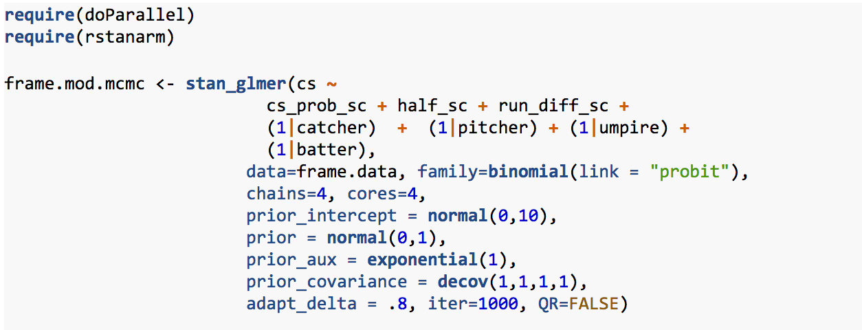
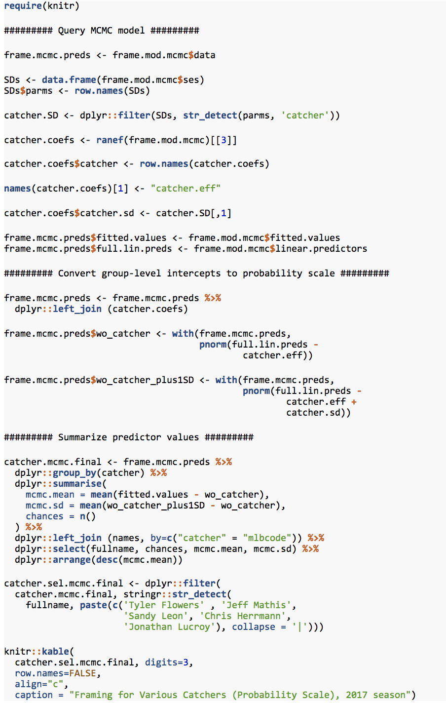
First, we’ll load the R packages we need, and then extract from the above-referenced MCMC model:
Framing for Various Catchers (Probit Scale), 2017 season
| fullname | mean | 50% | mcse | sd | 2.5% | 97.5% | n_eff | Rhat |
| Tyler Flowers | 0.296 | 0.296 | 0.001 | 0.036 | 0.225 | 0.367 | 1630 | 0.999 |
| Jeff Mathis | 0.140 | 0.141 | 0.001 | 0.046 | 0.051 | 0.228 | 1665 | 1.000 |
| Sandy Leon | 0.050 | 0.051 | 0.001 | 0.043 | -0.035 | 0.135 | 1525 | 1.000 |
| Chris Herrmann | -0.069 | -0.067 | 0.001 | 0.052 | -0.172 | 0.034 | 2000 | 1.000 |
| Jonathan Lucroy | -0.135 | -0.135 | 0.001 | 0.032 | -0.196 | -0.074 | 1405 | 1.000 |
Using the mean intercept for each player, we predict that the best framing catcher in baseball last season was Tyler Flowers (Braves). Jeff Mathis (Diamondbacks) was significantly above average, Sandy Leon (Red Sox) was just above average, Chris Herrmann (also Diamondbacks) was just below average, and Jonathan Lucroy (Rangers, Rockies) was quite bad. The 50th percentile value, a/k/a the “median,” follows the mean in this table, and the two are essentially identical. The “mcse” is the Monte Carlo standard error, which is virtually nill. The standard deviation (sd) gives us one measure of uncertainty around the mean estimate for each player, followed by the 2.5% lower bound and 97.5% upper bound of that uncertainty, also known as the 95th percentile uncertainty interval. Of note is that both ends of the 95th percentile intervals equal about 1.96 times the respective SDs. Combined with the virtual identity of mean and median, this means that the posterior around our group-level parameters is essentially normal. This simplifies our task considerably later on, as the mean and SD can fairly characterize the entire posterior for our parameters of interest. (Hold that thought). Finally, the table shows that we have a large number of “effective” samples, and that our Rhat values are essentially 1, both of which are consistent with convergence and reliable estimates.
That said, these numbers are not useful to us in their current form, because they are on the continuous probit scale, rather than the discrete probability scale between 0 (called ball) and 1 (called strike), which is what we were trying to model. To convert these values to probabilities above average, we need to take the average of the differences between the predicted outcomes of each pitch with and without each participant. RStan struggles a bit generating a predictive posterior with data set this large, so in lieu of that, we’ll query the fitted values and standard errors of our parameters, which were pre-calculated and saved by the model:
Framing for Various Catchers (Probability Scale), 2017 season
| fullname | chances | mcmc.mean | mcmc.sd |
| Tyler Flowers | 5348 | 0.036 | 0.004 |
| Jeff Mathis | 3241 | 0.016 | 0.005 |
| Sandy Leon | 4946 | 0.006 | 0.005 |
| Chris Herrmann | 2417 | -0.008 | 0.006 |
| Jonathan Lucroy | 6854 | -0.016 | 0.004 |
(In reality, taking the mean of the predicted differences with and without the SD is just a convenience function: the SD is essentially the same for all observations involving the same player, and we could just as well sample the difference from one row and be done with it.)
Although our table above labels it mcmc.mean, at BP we publish this metric as “Called Strikes Above Average” or “CSAA.” We typically report CSAA to three decimal points (e.g., 3.6%), beyond which the additional precision doesn’t translate into meaningful differences in runs. Because we are comparing methods in this paper, mean CSAA calculated by MCMC is described as mcmc.mean and the uncertainty is mcmc.sd. We will follow a similar convention in describing other methods below.
B. The Search for Shortcuts
As noted above, despite its superior results, MCMC tends to come at a heavy price: time. In our particular application, the problem is that we are expected to post updated results each morning from the previous night’s games, and, particularly given the other processes and models that need to run also, we can rarely spare more than an hour for a framing model to run, if that. For the first few weeks, MCMC could still be used. But once the sample sizes go north of 50,000 observations (about one month into the season), we are well past our permitted amount of time, even with parallel chains and modern hardware. If we want daily uncertainty estimates, we need to find an alternative, even if it isn’t quite as accurate as MCMC, that at least allows us to get close to what MCMC would report if it were run.
Almost most of you don’t run a sports statistic website, some version of this problem exists for anybody who performs statistical inference on a deadline. Perhaps you have only a half day to fit a model which ordinarily takes days, or 30 minutes to handicap the effect of some updated data before your business window closes. Sometimes you just don’t have time for MCMC, but still want to have the benefit of Bayesian uncertainty estimates. What do you do then?
1. Posterior Simulation
The quickest and easiest alternative is posterior simulation. Championed by Gelman and Hill, and provided in the sim function of Gelman and Su’s arm package for R, posterior simulation draws from a multivariate normal distribution and multiplies those values by the model’s covariance matrices to provide a simulated model posterior in very little time. Thus, when it works, posterior simulation adds only a few minutes to a lme4 model that itself takes at most about 10 minutes: well within our constraints.
Although the arm function states that it works directly with lme4, the merTools package makes sim a bit more user friendly. Using the RESim function from merTools, R draws the number of requested samples, which usually stabilize well before 1000. Let’s perform posterior simulation and compare the results to those from MCMC.
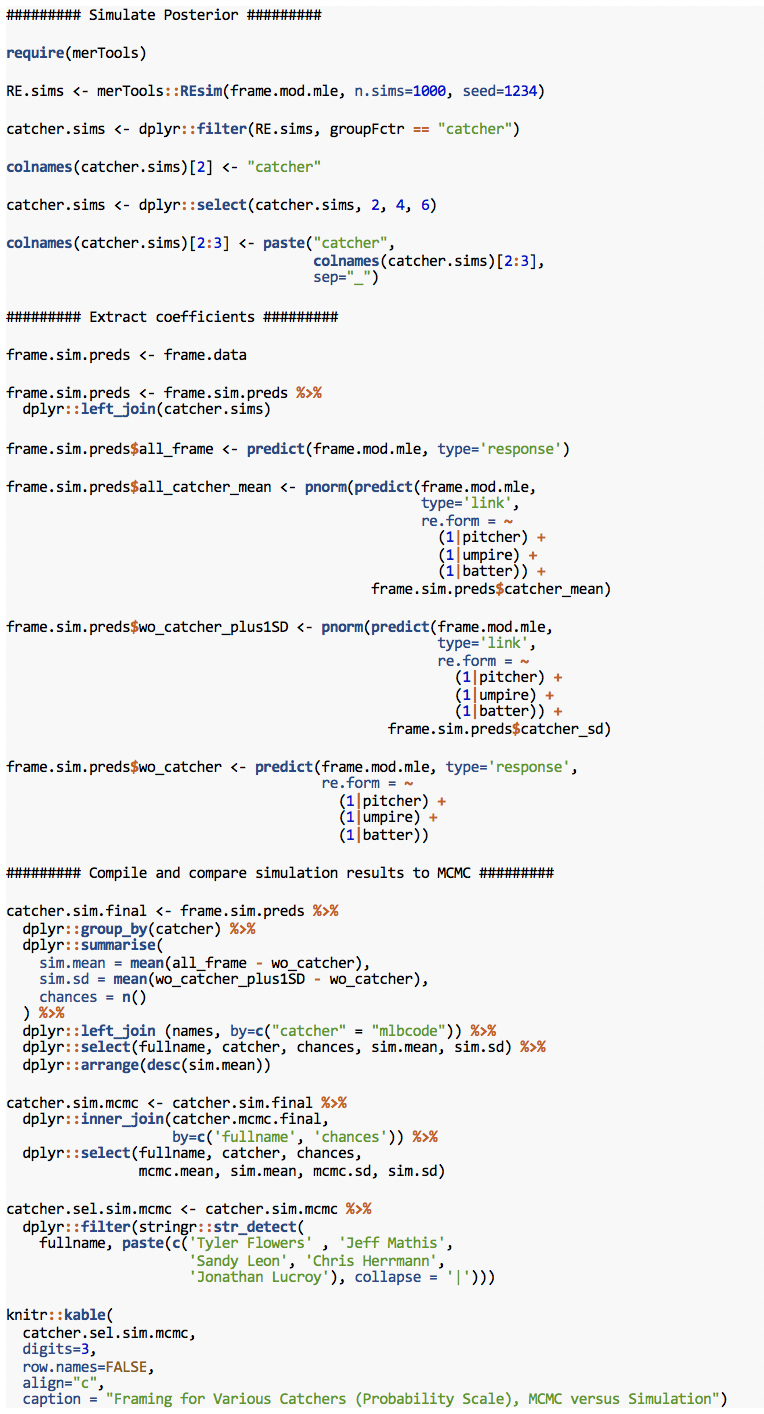
Framing for Various Catchers (Probability Scale), MCMC versus Simulation
| fullname | catcher | chances | mcmc.mean | sim.mean | mcmc.sd | sim.sd |
| Tyler Flowers | 452095 | 5348 | 0.036 | 0.036 | 0.004 | 0.008 |
| Jeff Mathis | 425772 | 3241 | 0.016 | 0.016 | 0.005 | 0.007 |
| Sandy Leon | 506702 | 4946 | 0.006 | 0.006 | 0.005 | 0.005 |
| Chris Herrmann | 543302 | 2417 | -0.008 | -0.008 | 0.006 | 0.010 |
| Jonathan Lucroy | 518960 | 6854 | -0.016 | -0.016 | 0.004 | 0.009 |
This method is problematic. The mean values reported by penalized likelihood are fine. But unlike the SDs from MCMC, which at least substantially correspond to the sample size provided by each catcher (“chances”), the simulated SDs are all over the place. Some of the SDs are the same as MCMC; players at the tails of the distribution though (Flowers, Lucroy) have their SDs doubled to .008+ from the .004 reported by MCMC, and Chris Herrmann, close to the mean, has a similar problem.
Misdiagnosing uncertainty by a factor of 2 is not acceptable. This is particularly true for posterior simulation, which only accounts for uncertainty in the non-group variables, not the grouped parameters or the model itself. A person looking at the results of posterior simulation, then, would reasonably assume that the incorrect doubling of the SDs was itself a conservative estimate of the actual uncertainty. In reality, MCMC accounts for all of this, and reports much smaller and more sensible intervals.
Posterior simulation is fine for simpler problems, but it appears to be a poor fit for a model with this level of complexity. Let’s try something else.
2. Variational Inference
Variational inference is the trendy way to perform Bayesian inference on data sets and/or models that are too challenging for MCMC sampling, either due to number of observations, intractability of the likelihood, or both. Instead of sampling its way to the target distribution, variational inference tries to find the closest multivariate normal distribution (via the K-L divergence) that will approximate the posterior distribution, using gradient descent. It is a clever idea that has been around for a while and will continue to become more useful as computing power grows. When it does work, ADVI is fairly efficient, providing a fully-Bayesian approximation of a model posterior within minutes. But ADVI also experimental and understandably fussy.
Alas, for our purposes variational inference is also (quite literally) a poor fit — at least the automatic differentiating variational inference (ADVI) included with Stan. ADVI could not run the preferred, probit link of the model at all. ADVI could run a logit link version of the model, but only in so-called “meanfield” form, rather than “full rank.” Meanfield ADVI focuses on getting the mean values of the parameters approximately correct, whereas full rank ADVI tends to reasonably approximate both mean values and variance. For us, the entire point of performing inference on group parameters is to correctly ascertain their variance. Thus, accuracy that extends only to the “mean” values from the non-preferred link, which weren’t particularly accurate anyway, is of little use. ADVI will not help us.
3. Maximum A Posteriori (MAP) Estimation
Briefly, we’ll consider another option that needs to be used more: the blme package from Chung et al. Designed to help keep covariance parameters from succumbing to boundary conditions, blme is a wrapper around lme4 that permits the explicit addition of priors to both the group and non-group parameters. The result is maximum a posteriori (MAP) estimates if you employ the priors, and the same penalized maximum likelihood estimates from lme4 if you turn the priors off. It is possible that the priors in blme, although still converging to point estimates only, may be helpful if they can steer the estimates in the correct direction sooner.
Alas, this approach is not meant to be either. Working from the probit units, look at the difference between the untransformed parameter ranges estimated by Stan and lme4 versus blme, for which we used the default parameters:
Group Variance Comparison: MCMC, MLE, and BLME
| group | mcmc.estimate | mle.estimate | blme.estimate |
| batter | 0.09 | 0.09 | 0.12 |
| pitcher | 0.11 | 0.11 | 0.09 |
| catcher | 0.12 | 0.12 | 0.95 |
| umpire | 0.11 | 0.10 | 0.99 |
While the Stan / MCMC and lme4 / MLE variance estimates are identical, the blme estimates range from slightly off to completely screwy. The culprit presumably is the default gamma / wishart covariance prior that blme employs to keep group intercepts away from zero; here, those priors appear to be overly influential and cause substantially less accuracy. It is possible the default covariance prior could be improved upon, but we already know that the default lme4 implementation requires no similar prior to get the variance parameters substantially correct, and if there is no need for a covariance prior, there is really no need for blme (Note: any priors placed on the non-group variables wash out regardless, because the data set is so large).
The covariance prior used by blme is actually similar in spirit to the group correlation prior used by Stan above; the problems seen here underscore that proper Bayesian inference is hard to do within a point estimate framework, which is why MCMC sampling is usually preferred.
III. A Bayesian Block Bootstrap Aggregator
Having considered various alternatives, let’s look at an updated version of an old friend: bootstrapping. Specifically, we can randomly resample the underlying data with replacement, re-run a penalized likelihood model in lme4 on each resampled data set, and compile a posterior consisting of all the group-level parameters participants estimated from these resampled data sets.
Bootstrapping is of course a standard tool of frequentist, rather than Bayesian statistics, and may seem rather rich for me, having banged on confidence intervals above, to be endorsing a frequentist resampling mechanism now. But a posterior is a posterior, and there is a generally-accepted Bayesian analogue to the frequentist bootstrap that treats the underlying data as a prior distribution, and thereby allows the creation of the aggregate posterior of parameter values that we seek.
A. The General Idea
The resampling portion of our approach involves treating the underlying data as discrete, as represented by a Dirichlet distribution. To query that distribution, we randomly sample from a unit exponential distribution to assign weights to each observation in the Dirichlet, and then in turn sample from the Dirichlet using the weights. We continue on, running the model on each resampled data set and compile our posterior by adding the transformed group-level intercepts from each modeled set of data at the conclusion of each sampling loop. The analysis remains philosophically Bayesian because (1) the data was resampled in a Bayesian manner and (2) lme4 is applying what amounts to a grand, unit-normal (if somewhat latent) prior over all the modeled resamples of the members represented within the various groups. Moreover, “[a]ll multilevel models are Bayesian in the sense of assigning probability distributions to the varying regression coefficients.” [Gelman and Hill, Kindle Locations 9667-9668]
We adopted this method because it made intuitive sense, but it really is not “new.” A similar approach was proposed here, although Dr. Graham’s proposal does not involve bootstrapping a multilevel model. For those familiar with machine learning, our approach is a form of “bootstrap aggregation” or “bagging.” Bagging, and so-called “ensemble models” in general, are more commonly associated with non-parametric modeling techniques like RandomForest. However, bagging can also be effective in aggregating ordinary regression estimates to provide better predictions and to capture uncertainty. In other words, while our approach is somewhat novel in this application, the underlying principles are fairly well established.
B. Resampling in Blocks
The method described just above is fine for ordinary Bayesian bootstrap resampling and should generally work for our application. One potential problem, though, is that raw (or “naive”) bootstrap resampling would treat every possible combination of pitches as equally likely to occur, when in fact that is obviously not true.
The sequence of pitches thrown during a plate appearance is a function of, among other things, the count in which those pitches are thrown. In two-strike counts, for example, pitchers will often throw out of the strike zone in an effort to draw a low-risk swing. In a three-ball count, on the other hand, most pitchers are loath to walk the batter, and will feel compelled to throw their pitch at least partially in the strike zone. This resulting difference in called-strike probability is visually apparent when you plot the densities of called-strike probabilities from these contrasting classes of pitch counts:
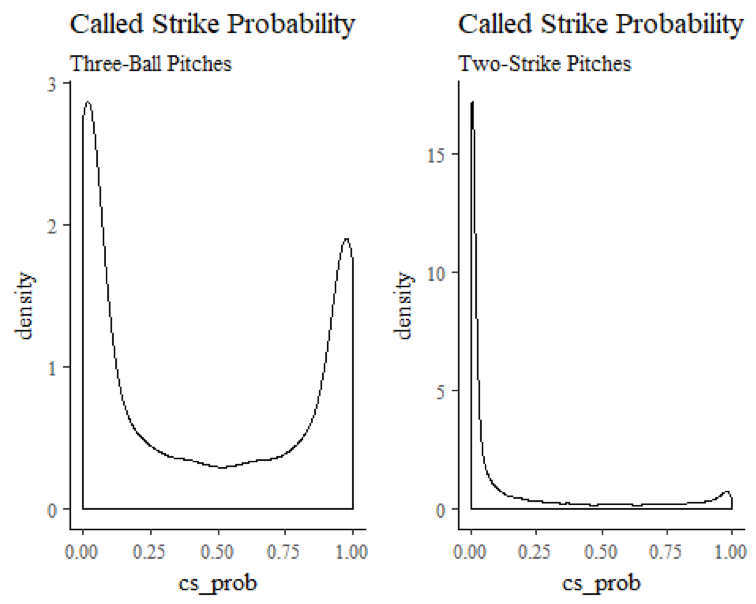
Why is this relevant? Well, once your data set gets sufficiently large, it may not matter much at all. But particularly when early-season samples are smaller, if you treat all pitches as equally likely, it is possible to end up with pitcher samples that disproportionately reflect one type of count, as opposed to the ebb and flow of called strike probability that proceeds over the course of an at-bat. If this happens, you could end up with samples that contain extreme and unrealistic results.
Outlier parameter samples are a particular concern in our application, because our goal is efficiency: getting accurate estimates as quickly as possible with as few resamples as possible. Even one outlier run will not only lower accuracy, but could require many, many more additional samples to push the outlier estimate out toward the tails of the posterior where it belongs (to the extent it belongs anywhere at all). We just don’t have time for that, and to the extent any resampled data fails to replicate overall plate appearances, which is how pitches always occur, said data set is worthless for our inference anyway.
The solution is to perform so-called “block sampling” — sample pitches from the distribution only in blocks of individual plate appearances, generally taking either all of the pitches from a plate appearance or none. We continue sampling in blocks until we achieve the size of the original sample. This requires a slight adjustment to our sampling strategy, but not much of one: this time we put the random weights on the various plate appearances in a data set, and randomly sample from those groups instead of from all pitches individually. The block sampling approach takes at most another few seconds to perform, and helps ensure that our samples will be substantially representative of actual plate appearances without any real downside.
C. The Bayesian Block Bootstrap
Enough talking: let’s see the code for our proposed Bayesian Bagging method, and then we’ll discuss the results.
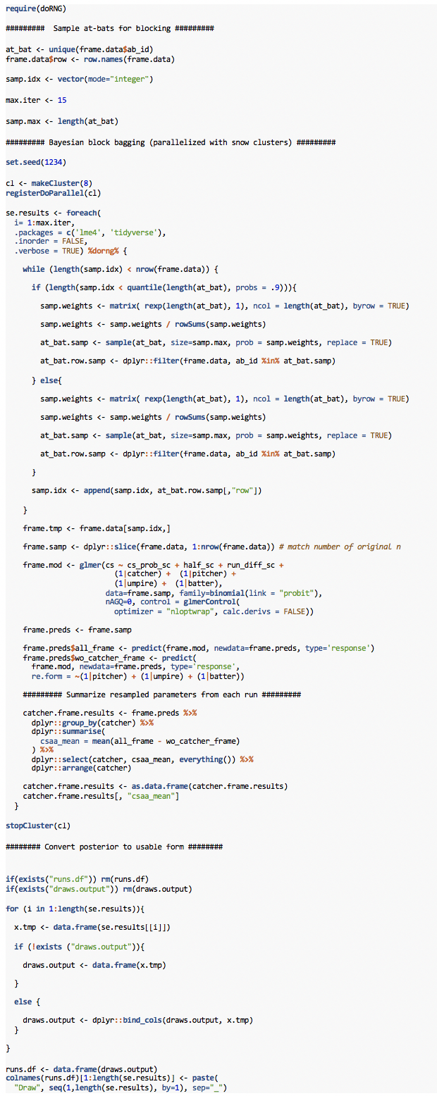
In sequence, we (1) separate out the at-bats a/k/a plate appearances so we can sample based on them and filter the data based on the sampled at-bats; (2) set the sampling procedure so it continues sampling until it has enough at-bats to provide the same number of pitches as the original sample; and then (3) finally matches the original number of observations exactly. An at-bat or two may end up truncated during this “true-up” process but otherwise plate appearances should remain intact.
Each resample is then run through the lme4 model and the results are compiled each time as noted above. You’ll note that we made a few tweaks to speed up the modeling: (1) we switched off the Laplace Approximation and went with instead with nAGQ=0, which is slightly less accurate but also faster and sufficiently accurate for our purposes; (2) we switched to a faster optimizer, NLOPT; (3) we told lme4 not to waste time calculating derivatives, because for this application nobody cares.
Because these resamples all follow the same process, we parallelize them. This code uses snow clusters for cross-platform compatibility (Mac / Unix users can obviously fork instead if they prefer, and have sufficient memory).
Lastly, we convert the parallelized output into a posterior data frame (runs.df) that I at least find better suited to summarization.
D. The Results
Does Bayesian Bagging work? At first glance, you may think not. Look, for example, at the posterior for Framer Extraordinaire Tyler Flowers, for which we’ve provided density plots in progressing increments. Are we quickly finding our normal posterior?
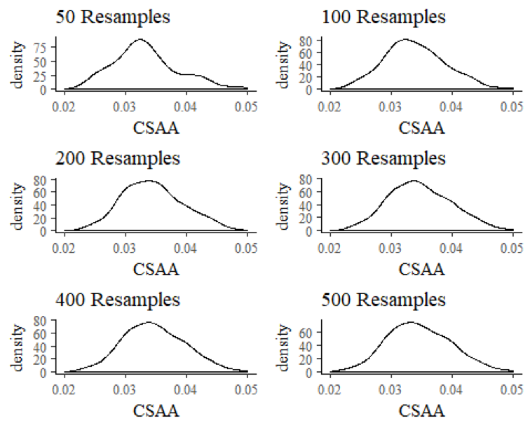
Hmm. After 500 repetitions, we seem to be approaching normality, although there is still some skew to the distribution. But if we are waiting for the exact replica of the MCMC posterior, it appears we are going to be waiting for a while. That’s a problem because even at 10 minutes per model, with 8 cores, 500 repetitions would take about 5 hours. That’s essentially like waiting for MCMC, and is not going to get it done.
Except! We have a shortcut, and a critical one at that. We already know that the posterior is normally distributed from our analysis of the MCMC posterior above. That means, by definition, that we can completely characterize the posterior distribution with the mean and standard deviation alone. We know that the mean estimates provided by lme4 are correct in this application (see the simulation results above), and we also know the approximate standard deviations around those estimates from our MCMC simulation. Thus, we don’t need to perfectly replicate our desired MCMC posterior; the only thing we need to do is to get reasonably accurate estimates of what the standard deviations would be around the means if we did have unlimited time to run the bagging algorithm. As it turns out, these estimates become reasonably accurate very quickly.
Take, for example, the estimated standard deviation of catcher CSAA after a mere 25 resamples, and compare it to the MCMC and posterior simulation results. We’ll describe the Bagging SD as “BayesBag.sd”:
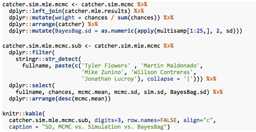
SD, MCMC vs. Simulation vs. BayesBag
| fullname | chances | mcmc.mean | mcmc.sd | sim.sd | BayesBag.sd |
| Tyler Flowers | 5348 | 0.036 | 0.004 | 0.008 | 0.005 |
| Martin Maldonado | 8267 | 0.019 | 0.004 | 0.007 | 0.004 |
| Mike Zunino | 6961 | 0.007 | 0.004 | 0.004 | 0.004 |
| Willson Contreras | 6228 | -0.004 | 0.004 | 0.004 | 0.004 |
| Jonathan Lucroy | 6854 | -0.016 | 0.004 | 0.009 | 0.004 |
While Bayesian Bagging SD estimates are not identical to MCMC, they are quite close, and much closer than posterior simulation. That is confirmed when we compute the weighted root mean square error (wRMSE) of the two approaches, as compared to full MCMC:
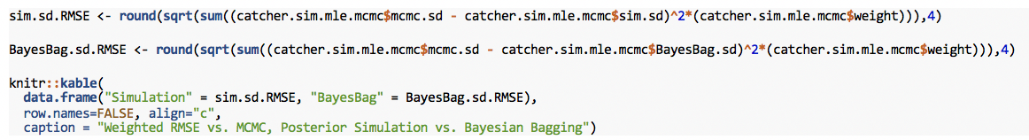
Weighted RMSE vs. MCMC, Posterior Simulation vs. Bayesian Bagging
| Simulation | BayesBag |
| 0.0034 | 0.0013 |
Bayesian Bagging is almost three times more accurate, on average, than posterior simulation. With CSAA being meaningful only to three significant figures, a rounded accuracy of .001 is therefore more than sufficient. Furthermore, with multiple cores, Bayesian Bagging achieves this within about 30 to 45 minutes for our framing model, even with a full season of data (300,000+ observations) — a significant improvement over the time required for full MCMC.
This demonstrates that Bayesian Bagging can be a worthwhile method for quickly approximating Bayesian uncertainty of group-level parameters.
E. Limitations
This analysis was aided by several factors that should not be taken for granted in efforts to apply Bayesian Bagging to other settings.
First, we actually completed full, MCMC-sampled Bayesian inference on our data set before proceeding to verify that bagging MLE models was a worthwhile substitute. Do not assume that MLE can adequately model your uncertainty without first confirming what that uncertainty most likely is.
Second, your posterior may not end up being normally distributed, even if your group-level parameters have a unit-normal prior distribution being applied to them. If your posterior is not normally distributed, Bayesian Bagging still is an option, but you then need to decide the actual interval you care about and confirm sufficient accuracy with that interval. Achieving reasonable estimates of the tails of a distribution takes somewhat longer than the SD, but the estimates, at least with framing models, can still approach reasonableness within 40 or 50 resamples, and sometimes sooner.
Third, as with all forms of Bayesian inference, domain knowledge trumps all. The primary reason we conceived of, implemented, and confirmed the usefulness of this method for our application is because catcher framing models are something we know very well. If you are unfamiliar with your subject, the odds of making a disastrous assumption go up dramatically. Educate yourself about what your subject matter first, or get help from somebody who can help you.
Conclusion
We hope you find this method useful, and that sports websites, as well as others, can use the methods described to swiftly estimate uncertainty for posted statistics when full MCMC is not a feasible option.
Special thanks to Rasmus Bååth, Ron Yurko, the Stan team, the BP Stats team, and especially to Rob Arthur, who kept insisting that this method be better.
Additional References
Andrew Gelman and Yu-Sung Su (2016). arm: Data Analysis Using Regression and Multilevel/Hierarchical Models. R package version 1.9-3. https://CRAN.R-project.org/package=arm
Chung Y, Rabe-Hesketh S, Dorie V, Gelman A and Liu J (2013). “A nondegenerate penalized likelihood estimator for variance parameters in multilevel models.” Psychometrika, 78(4), pp. 685-709. http://gllamm.org/
Douglas Bates, Martin Maechler, Ben Bolker, Steve Walker (2015). Fitting Linear Mixed-Effects Models Using lme4. Journal of Statistical Software, 67(1), 1-48. doi:10.18637/jss.v067.i01.
Gelman, Andrew; Hill, Jennifer. Data Analysis Using Regression and Multilevel/Hierarchical Models (Analytical Methods for Social Research) . Cambridge University Press. Kindle Edition. 2007.
Jared E. Knowles and Carl Frederick (2016). merTools: Tools for Analyzing Mixed Effect Regression Models. R package version 0.3.0. https://CRAN.R-project.org/package=merTools
Long, Christopher. Mixed Models in R – Bigger, Faster, Stronger. 2015.
R Core Team (2017). R: A language and environment for statistical computing. R Foundation for Statistical Computing, Vienna, Austria. https://www.R-project.org/
Stan Development Team (2016). rstanarm: Bayesian applied regression modeling via Stan. R package version 2.13.1. http://mc-stan.org/
Vehtari A, Gelman A and Gabry J (2016). “loo: Efficient leave-one-out cross-validation and WAIC for Bayesian models.” R package version 1.1.0, https://CRAN.R-project.org/package=loo
Thank you for reading
This is a free article. If you enjoyed it, consider subscribing to Baseball Prospectus. Subscriptions support ongoing public baseball research and analysis in an increasingly proprietary environment.
Subscribe now
The question you pose at the beginning -- the meaning of the difference between 8.3 and 8.1 WAR -- is something I have no real answer to myself, and thinking about it, I really just decide whether I think there is a significant difference between two value estimates such as WAR based on gut-feel. I would love some uncertainty intervals or standard deviations with my sabermetrics. Such numbers would give much more intuition as to the precision of an estimate, give an understanding as to how the precision of an estimate changes as sample size increases and other factors change, as well as allow me to establish with more confidence whether a difference in value is statistically significant or not.
Do you think, when this information becomes available, that it will integrate itself into standard analysis in the online community? Writers feeling obligated to explain how distributions work every time they cite a standard deviation might hinder even statistically inclined writers from using these numbers regularly. But I might be totally wrong about that, and I hope so.